Impulse Response and Convolution

Impulse Response and Convolution#

This reading develops one of the most important ideas in signals and systems: the impulse response. The impulse response provides a complete description of a linear time-invariant (LTI) system. Once it is known, the system’s response to any input can be determined using convolution.

The goal here is not only to present the formulas, but to build strong intuition for why convolution arises naturally from linearity and time invariance.

1. Why the Impulse Response Is Fundamental#

In many engineering systems - electrical circuits, mechanical systems, control systems, and signal processing algorithms — we are interested in understanding how a output signal depends on an input signal. For example, we may want to predict how the voltage across a circuit responds to an applied current, how the position of a mechanical structure responds to a force, or how a digital filter modifies an incoming sequence of samples.

For a general system, the relationship between input and output can be extremely complicated. It may depend on nonlinear effects, memory, or changes in system parameters over time. However, for linear time-invariant (LTI) systems, there is a remarkable and powerful simplification:

Important

An LTI system is completely characterized by its impulse response.

This means that if we know how the system responds to a single, idealized input called an impulse, then we can determine how the system responds to any input signal. Rather than analyzing the system separatly for every possible input, we only need to understand one special response.

The impulse response can be thought of as the system’s fingerprint. It captures how the system reacts over time, including delays, smoothing effects, oscillations, and decay. Much of signals and systems theory is built around learning how to use this fingerprint to predict system behavior.

To understand why the impulse response plays such a central role, we proceed in three steps:

Define impulse signals and their key properties
Show how arbitrary signals can be constructed from impulses
Use linearity and time invariance to compute the output

Each step relies directly on the defining properties of LTI systems.

2. Discrete-Time Impulse Response#

We begin with discrete-time systems, since impulses and summations are easier to visualize and manipulate mathematically. The ideas developed here will later extend naturally to continuous time systems.

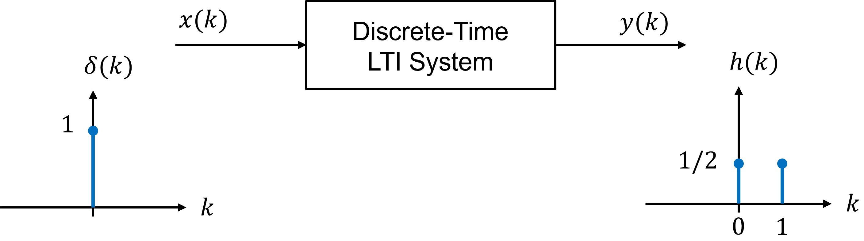
_images/LTI_System.png — Fig. 1 Block diagram of a discrete-time LTI system showing input \(x(k)\), output \(y(k)\), impulse input \(\delta(k)\), and impulse response \(h(k)\).#

Fig. 1 illustrates the basic input–output relationship of a discrete-time LTI system. It emphasizes that the impulse response \(h(k)\) is defined as the system output when the input is the unit impulse \(\delta(k)\). This definition forms the foundation for all later analysis.

2.1 The Unit Impulse (Kronecker Delta)#

The unit impulse, also called the Kronecker delta, is defined as

\[\begin{split} \delta(k) = \begin{cases} 1, & k = 0 \\ 0, & k \neq 0 \end{cases} \end{split}\]

Although this signal may appear artificial at first, it plays a role similar to that of a basis vector in linear algebra. Just as basis vectors allow us to represent any vector as a weighted sum, impulse signals allow us to represent any discrete-time signal as a weighted sum of shifted (or delayed) impulses.

When the input to the system is the unit impulse, the output is called the impulse response:

\[ \delta(k) \longrightarrow h(k). \]

The impulse response describes how the system behaves when it is excited at a single instant in time. It reveals essential properties of the system’s dynamics.

2.2 Time Invariance: Shifting the Impulse#

A system is time-invariant if delaying the input by some amount produces an identical delay in the output. Mathematically, if

\[ \delta(k) \longrightarrow h(k), \]

then for any integer \(n\),

\[ \delta(k-n) \longrightarrow h(k-n). \]

This property ensures that the system’s behavior does not depend on when the input is applied, but only on the relative timing between inputs. Time invariance allows us to predict system behavior at all times using a single impulse response.

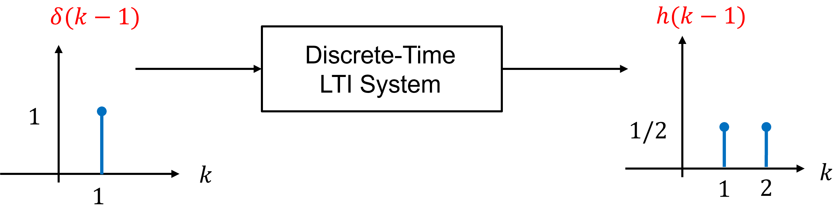
_images/DelayedImpulseResponse.png — Fig. 2 Illustration showing that a delayed impulse input \(\delta(k−n)\) produces a delayed output \(h(k−n)\).#

Fig. 2 demonstrates the time-invariance property visually. When the impulse input is shifted (or delayed) in time, the output shifts (or delays) by exactly the same amount.

2.3 Linearity: Scaling the Impulse#

A system is linear if it satisfies two properties:

Scaling: Scaling the input scales the output
Additivity: The response to a sum of inputs is the sum of the responses

For scaling,

\[ a\delta(k) \longrightarrow a h(k). \]

This proportional response is essential for constructing the output corresponding to more complicated inputs.

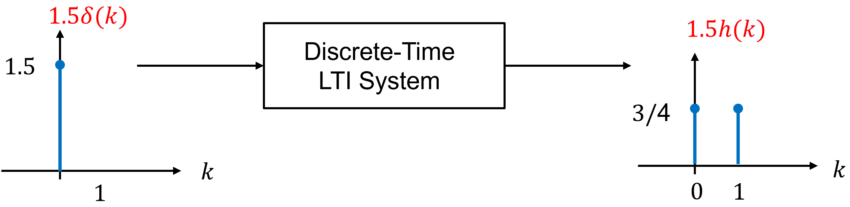
_images/ScaledImpulseResponse.png — Fig. 3 Illustration demonstrating scaling: input \(a\delta(k)\) produces output \(ah(k)\).#

Fig. 3 illustrates linearity through scaling. Increasing the amplitude of the impulse increases the amplitude of the response by the same factor, reinforcing the proportional nature of linear systems.

3. Decomposition of Discrete-Time Signals#

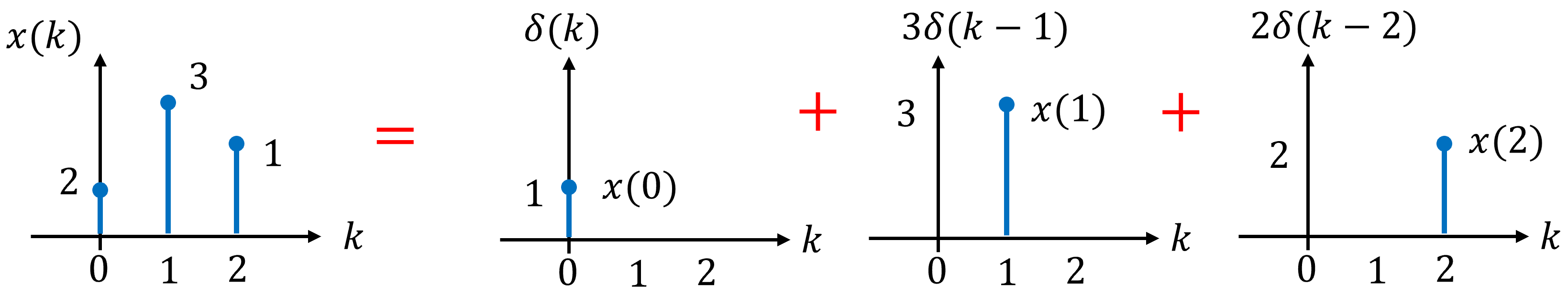
_images/ImpulseDecomposition.png — Fig. 4 Example discrete-time signal decomposed into scaled and shifted impulse signals.#

Fig. 4 shows how an arbitrary discrete-time signal can be expressed as a sum of weighted and shifted impulses. Each impulse corresponds to one sample of the signal, making the decomposition visually concrete.

The key insight that leads directly to convolution is that any discrete-time signal can be constructed from shifted impulses.

Let \(x(k)\) be an arbitrary discrete-time signal. Then it can be written as

\[ x(k) = \sum_{n=-\infty}^{\infty} x(n) \delta(k-n). \]

Although this expression may initially appear more complicated than the original signal, it has a clear interpretaiton. Each impulse \(\delta(k-n)\) isolates the signal value at time index \(n\), and the coefficient \(x(n)\) specifies the strength of that impulse.

In this sense, the impulse acts as a sampling operator, extracting individual samples of the signal and placing them at the correct time locations.

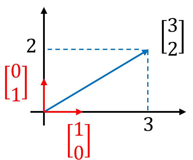
_images/BasisVectors.png — Fig. 5 Basis vectors#

This idea is closely related to expressing a vector as a linear combination of basis vectors. For example, consider a vector \(\begin{bmatrix} 3 & 2 \end{bmatrix}^\top\) as illustrusted in Fig. 5. This vector can be decomposed as

\[\begin{split} \begin{bmatrix} 3 \\ 2 \end{bmatrix} =3\begin{bmatrix} 1 \\ 0 \end{bmatrix} + 2\begin{bmatrix} 0 \\ 1 \end{bmatrix}. \end{split}\]

Here, the unit vectors form a basis for \(\mathbb{R}^2\). Similarly, shifted impulse signals form a basis for discrete-time signals. From this perspective, convolution emerges naturally as the process of combining the system’s responses to each basis element.

4. Discrete-Time Convolution#

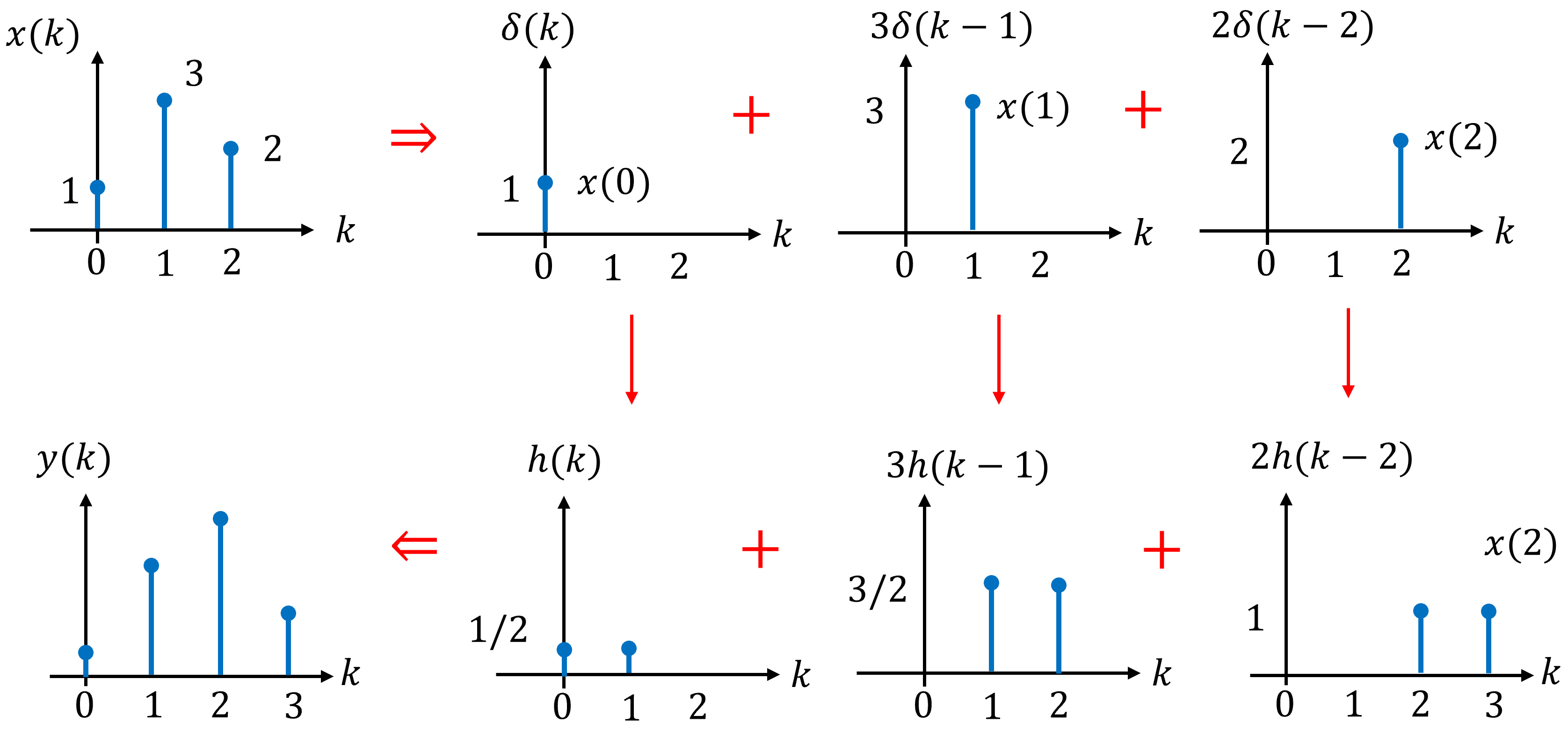
_images/DiscreteConvolution.png — Fig. 6 Convolution is visualized as a superposition of weighted and shifted impulse responses.#

Fig. 6 illustrates the key idea behind discrete time convolution: the output of an LTI system is formed by adding together many delayed and scaled copies of the system’s impulse response. To see how this works in detail, consider the discrete-time input signal \(x(k)\) shown in Fig. 6. As discussed in the previous section, any discrete-time signal can be expressed as a sum of weighted and shifted unit impulses. For this particular signal, we may write

\[ x(k) = \delta(k) + 3\delta(k-1) + 2\delta(k-2). \]

This expression states that the signal consists of three impulses: one at \(k=0\), one at \(k=1\) with weight 3, and one at \(k=2\) with weight 2. Each impulse represents the value of the signal at a specific time index. More generally, we can rewrite this expresion using the signal values \(x(n)\) as coefficients:

\[ x(k) = x(0)\delta(k) + x(1)\delta(k-1) + x(2)\delta(k-2). \]

Writing the signal in this form is useful because it makes the role of each impulse explicit: every term in the sum corresponds to one sample of the input signal.

Response of an LTI System to the Decomposed Input#

Once the input signal has been decomposed into impulses, computing the system output becomes straightforward. By definition, the response of an LTI system to a unit impulse is the impulse response \(h(k)\). Due to time invariance, a shifted impulse produces a shifted impulse response:

\[ \delta(k-n) \longrightarrow h(k-n). \]

Furthermore, because the system is linear, scaling the impulse scales the output by the same factor. Therefore, the response to the term \(x(n)\delta(k-n)\) is

\[ x(n)\delta(k-n) \longrightarrow x(n)h(k-n). \]

Applying this reasoning to each impulse in the decomposition of \(x(k)\), the total output is obtained by summing the individual responses. For our example signal, the output is

\[ y(k) = h(k) + 3h(k-1) + 2h(k-2), \]

which can also be written as

\[ y(k) = x(0)h(k) + x(1)h(k-1) + x(2)h(k-2). \]

This expression makes the structure of the output clear: it is formed by adding together shifted copies of the impulse response, each weighted by the corresponding input sample.

Using summation notation, we can write this result compactly as

\[ y(k) = \sum_{n=0}^{2} x(n)h(k-n). \]

General Convolution Sum#

The same reasoning applies to any discrete-time input signal, not just this finite-length example. Since any signal can be expressed as a sum of weighted impulses over all time indices, the output of an LTI system is given by

\[ y(k) = \sum_{n=-\infty}^{\infty} x(n)h(k-n). \]

This summation is called discrete-time convolution. It describes how the input signal \(x(k)\) and the impulse response \(h(k)\) combine to produce the output.

We use the convolution operator * to write this relationship more compactly:

\[ y(k) = (x * h)(k). \]

Interpretation#

Discrete-time convolution can be interpreted as a superposition process. Each sample of the input signal generates a shifted and scaled copy of the impulse response, and the output at any time \(k\) is the sum of all these contributions. In other words, the impulse response acts as a template that is repeatedly shifted, weighted, and added according to the input signal.

Important

The output is formed by adding together many shifted copies of the impulse response, each weighted by the input signal.

Real-Life Analogy: Echoes and Convolution#

A helpful real-life analogy for discrete-time convolution is sound echo in a large room or a canyon. Imagine clapping your hands once. The sound you hear afterward—multiple delayed and gradually fading echoes—is analogous to the impulse response \(h(k)\) of the environment. A single clap acts like an impulse input, and the sequence of echoes reveals how the environment responds over time.

Now imagine clapping several times with different strengths and at different moments. Each clap produces its own set of echoes, delayed in time and scaled in amplitude according to how loud the clap was. What you actually hear is the sum of all these echoes overlapping in time. In this analogy, the claps correspond to the input signal \(x(k)\), the echoes correspond to shifted versions of the impulse response \(h(k-n)\), and the overall sound you hear corresponds to the output signal \(y(k)\).

This analogy highlights the key idea behind convolution: each input sample excites the system, producing a delayed and scaled response, and the final output is the sum of all such responses. Convolution is therefore not an abstract mathematical operation, but a natural way to describe how real systems accumulate the effects of past inputs over time.

5. Continuous-Time Impulse Response#

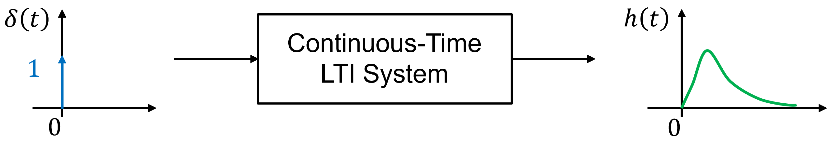
_images/LTI_System_CT.png — Fig. 7 Continuous-time LTI system responding to a Dirac delta input \(\delta(t)\) with impulse response \(h(t)\)#

Fig. 7 introduces the impulse response for continuous-time systems. The diagram closely mirrors the discrete-time case, emphasizing that the impulse response \(h(t)\) is defined as the system output when the input is the Dirac delta function \(\delta(t)\).

Conceptually, the idea of an impulse response does not change when moving from discrete time to continuous time. What changes is the mathematical machinery: sums become integrals, and sequences become continuous functions of time. The underlying logic, based on linearity and time invariance, remains exactly the same.

As before, the impulse response serves as a complete characterization of the system. Once \(h(t)\) is known, the system’s response to any continuous-time input can be computed using convolution.

5.1 The Dirac Delta Function#

The Dirac delta function \(\delta(t)\) is defined by the property

\[ \int_{-\infty}^{\infty} \delta(t)dt = 1. \]

Unlike ordinary functions, the delta function is zero everywhere except at \(t = 0\), where it is unbounded. For this reason, it is not a function in the traditional sense, but rather a generalized function (or distribution). Despite this mathematical subtlety, the Dirac delta is one of the most useful tools in signals and systems analysis.

Physically, the delta function models an input that delivers a finite amount of energy or impulse over an infinitesimally short time. Examples include an idealized hammer strike, a sudden force applied to a mechanical system, or a very short voltage pulse applied to a circuit.

When the input to a continuous time LTI system is the delta function, the output is defined to be the impulse response:

\[ \delta(t) \longrightarrow h(t). \]

The impulse response reveals how the system reacts immediately after being excited and how that effect evolves over time.

5.2 Decomposition of Continuous-Time Signals#

Any continuous-time signal \(x(t)\) can be expressed as

\[ x(t) = \int_{-\infty}^{\infty} x(\tau)\delta(t-\tau)d\tau. \]

This expression is the continuous-time counterpart of impulse decompositon in discrete time. Each shifted (or delayed) impulse \(\delta(t-\tau)\) isolates the value of the signal at time \(\tau\), while the coefficient \(x(\tau)\) determines the strength of that impulse.

Conceptually, this representation says that continuous-time signal can be constructed by stacking together infinitely many infinitesimal impulses. Each impulse contributes independently to the system output, and the total signal is formed by integrating over all such contributions.

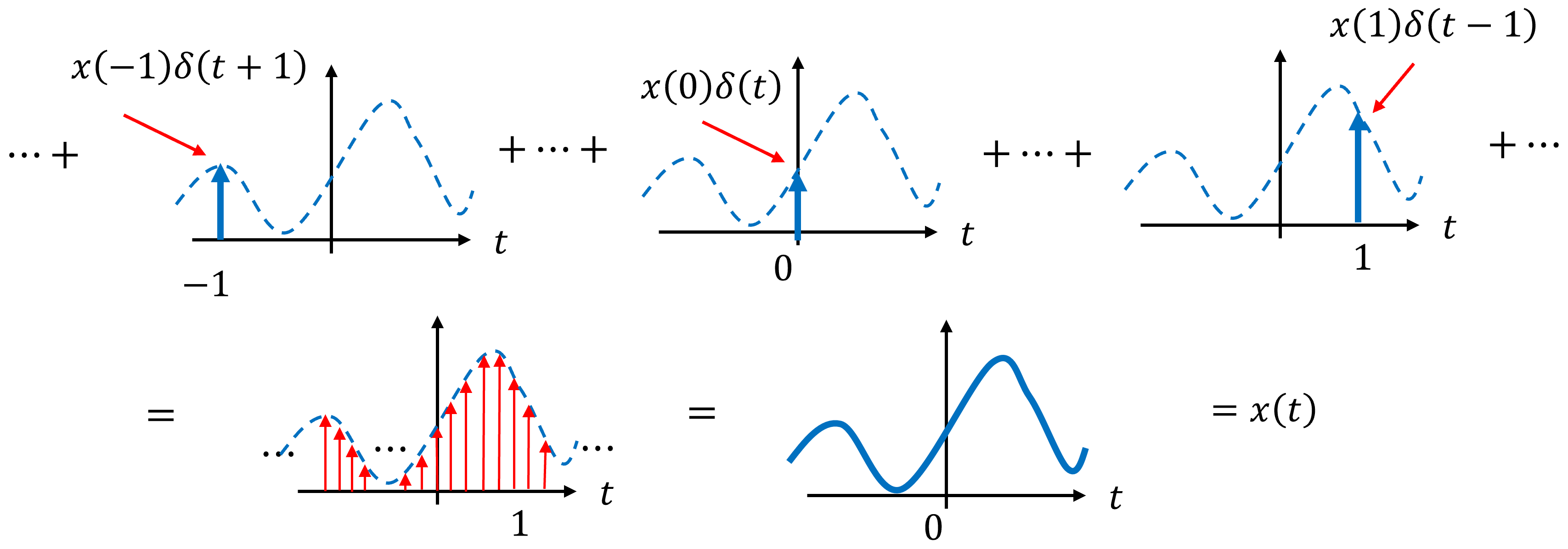
_images/ImpulseDecompositionCT.png — Fig. 8 Continuous-time signal represented as a superposition of shifted impulses.#

Fig. 8 illustrates a powerful way to think about continuous time signals as an infinite collection of impulses, each occurring at a different time and weighted by the signal’s value at that time.

6. Continuous-Time Convolution#

Using impulse decomposition together with linearity and time invariance, the output of a continuous-time LTI system is given by

\[ y(t) = \int_{-\infty}^{\infty} x(\tau) h(t-\tau) d\tau. \]

This expression is called the convolution integral. It states that each impulse occurring at time \(\tau\) produces a shifted impulse response \(h(t-\tau)\), scaled by the input value \(x(\tau)\). The output is the accumulation of all such responses over time.

Using the convolution operator, this relationship is written compactly as

\[ y(t) = (x * h)(t). \]

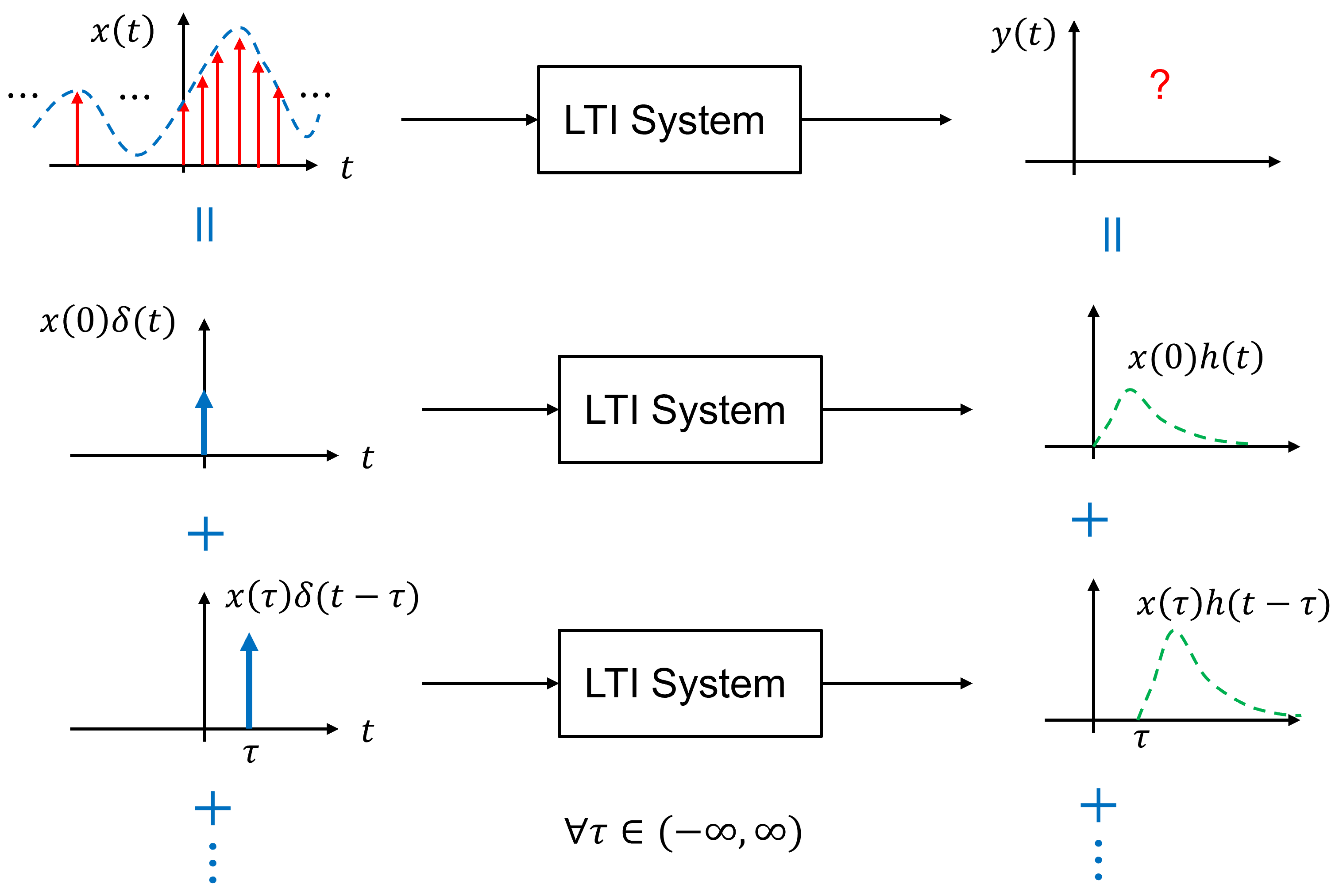
_images/ContinuousConvolution.png — Fig. 9 Graphical depiction of convolution as integration of shifted impulse responses weighted by the input signal.#

Fig. 9 connects the convolution integral to physical intuition. It shows that the output at time \(t\) is obtained by integrating shifted copies of the impulse response, each weighted by the input signal.

Note

Convolution provides a universal input–output relationship for all continuous-time LTI systems, regardless of their physical realization.

7. Discrete-Time vs. Continuous-Time#

Although discrete-time and continuous-time systems use different mathematical tools, their underlying concepts are identical. In both cases, signals are decomposed into impulses, system behavior is captured by an impulse response, and outputs are computed by superposition.

Concept	Discrete Time	Continuous Time
Impulse	\(\delta(k)\)	\(\delta(t)\)
Signal decomposition	Summation	Integral
Impulse response	\(h(k)\)	\(h(t)\)
System output	Convolution sum	Convolution integral

8. Key Takeaways#

The impulse response completely characterizes an LTI system in both discrete and continuous time.
Any signal can be decomposed into a superpostion of weighted, shifted impulses.
Linearity and time invariance allow system responses to be constructed through superposition.
Convolution describes how inputs are transformed into outputs by accumulating impulse responses over time.