Analog Filter Lab

Analog Filter Lab#

Build the R-C filter you analyzed in Objective 2.4 and measure its frequency response on a scope, swap the two components and identify what the circuit has become, then hypothesize and test a third circuit that goes past what Objective 2.4 analyzes.

At a glance

Run at Lesson 19. Work with your lab partner (groups of 2). The completed handout is submitted through Gradescope — the course’s system of record for submissions — by the end of the lab period, and is worth 1 project point. The midterm is also due at this lesson.

Lab Goal#

You will build and investigate filter circuits using the function generator, oscilloscope, and breadboard — then compare what you measure against what Objective 2.4 predicts.

Equipment#

Keysight 33500B waveform generator — the function generator, abbreviated FG on the handout
Tektronix 2 Series oscilloscope
Breadboard and mini-grabber cables — test leads with small spring-loaded clips that grip a component lead or a breadboard wire
\(R = 10\ \text{k}\Omega\) and \(C = 0.01\ \mu\text{F}\)
500 mH inductor — Part 7 only; a new component you have not used yet
ZLCR meter — an impedance / inductance / capacitance / resistance meter, used in Part 6 to measure the actual component values

Authorized Resources#

Lab equipment, your laptop, the handout, course slides and readings, practice problems, the equation sheet, and EI from instructors during the period. You may not use materials from previous semesters.

You may also use GenAI only up to Level 3 (use of GenAI as a feedback tool on student-generated work, as defined in the AW GenAI Policy).

Document any collaboration or GenAI use on the handout.

Part 1 — Configure the Function Generator (handout STEP 1–8)#

Program the generator for a 4 kHz, 10 V_pp sinusoid. V_pp is peak-to-peak voltage — the full swing of the waveform, from its lowest point to its highest.

Turn the function generator on and set the menu to CH1.
Press Output Load and set it to High Z.
Press Waveform and choose Sine.
Press Frequency and enter 4 kHz on the keypad.
Press Parameters, choose Amplitude, and set 10 V_pp.

You should see the CH1 status line reading Sine, HighZ, a frequency of 4.000000 kHz and an amplitude of 10.000 V_pp. The output is still off — that is correct for now.

Why High Z matters

Setting the output load to High Z is what makes the peak-to-peak amplitude you program equal the amplitude you measure. Leave it at 50 Ω and every reading will be off by a factor of two — and the error will look like a circuit problem rather than a setup problem.

Part 2 — Build the Filter and Predict (handout STEP 10–11, then STEP 9)#

Build the R-C circuit on the breadboard, with the output taken across the capacitor. Use the red mini-grabber to connect the function generator to the board.

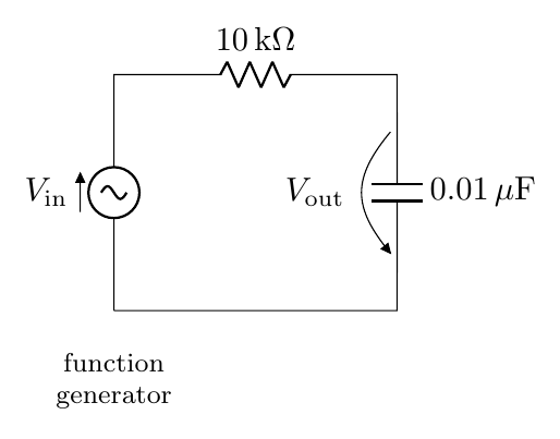
R-C low-pass filter: the function generator drives a 10 kΩ resistor in series along the top of the loop, and a 0.01 µF capacitor sits across the right-hand side, from the resistor's output node down to the ground return. The output voltage is taken across the capacitor.

Before you power anything, compute and record your predicted cutoff:

\[ f_{\text{cutoff}} = \frac{1}{2\pi RC} \]

You should see a prediction in the low kilohertz. If your number lands in the hertz or the megahertz, you have a unit-conversion error — find it before you build anything on top of it.

Connect CH1 of the scope where the generator meets your circuit, and CH2 across the capacitor. Make sure CH1’s black lead is at the bottom of the circuit.

Why the black lead has to go at the bottom

The scope’s black lead and the function generator’s black lead are both tied to earth ground through their power cords, so they are the same electrical node whether you intended it or not. Clip a black lead anywhere other than the bottom of the circuit and you connect that point straight to ground through the instruments, shorting out whatever sat between it and the bottom rail. The waveform collapses, and nothing on the breadboard looks wrong.

Only now, with the circuit built and both probes placed, turn the generator’s output on: Output → ON.

Part 3 — Configure the Oscilloscope (handout STEP 12–17)#

Turn CH1 and CH2 on; make sure the others are off.
Adjust the vertical scale so both channels’ maxima and minima are on screen.
Adjust the horizontal scale so about two cycles are displayed.
Press Measure and add Peak-to-Peak for both channels.
Press Measure again, select Time Measurements → Phase, set Source 1 to CH2 and Source 2 to CH1, then Add.

You should see two sine waves at the same frequency, and a measurement readout carrying two peak-to-peak values and one phase angle in degrees. If the phase reads as a wildly unstable number, the output waveform is too small for the scope to time reliably — turn CH2’s volts/div down so the trace fills more of the screen rather than trusting the number.

Part 4 — Measure the Frequency Response (handout STEP 18)#

Sweep the generator and complete the table. Keep both waveforms inside the scope window at every point, and keep the output large enough that the scope can still measure phase — adjust volts/div as needed.

Frequency	Input amplitude (V_pp)	Output amplitude (V_pp)	Phase difference (°)	Gain
100 Hz
200 Hz
400 Hz
1 kHz
? kHz				0.707
2 kHz
4 kHz
10 kHz
20 kHz
40 kHz

For the row between 1 and 2 kHz, hunt for the frequency where the gain is 0.707. That is your measured cutoff frequency.

You should see a gain close to 1 at the bottom of the sweep, holding roughly flat, then falling steadily once you push past the cutoff — by about a factor of ten for every factor of ten in frequency. The phase difference should march away from 0° in the same direction the whole way. If the gain never settles near 1 at the bottom of the sweep, re-check High Z and your probe placement before you record anything.

Then answer:

What type of filter is this?
What is its measured cutoff frequency?
Why is the measured cutoff not exactly what you predicted?

The phase gives you a second, independent confirmation: at the cutoff of this low-pass the reading should be ≈ −45° (and ≈ +45° for the Part 5 high-pass). If the gain says 0.707 but the phase is nowhere near 45°, you are not at the cutoff.

Where the plot and the percent difference go. The handout asks for both, in a Before you continue note at the top of its page 4 — immediately after the Part 4 blanks and just before STEP 19 — and gives you a place for them on its last page (page 6): a printed grid with a logarithmic frequency axis, and a blank for the percent difference. Plot gain versus frequency on that grid (a point for every row of your table, then a smooth curve through the points), mark the −3 dB point on it and label it with your measured cutoff frequency, and write the percent difference between your measured and predicted cutoff in the blank below the grid, with your work. Percent difference is

\[ \%\ \text{difference} = \frac{|f_{\text{measured}} - f_{\text{predicted}}|}{f_{\text{predicted}}} \times 100 \]

Measure the input at every frequency

Do not assume the input amplitude held steady as you swept. Generators sag under load, and an input you assumed rather than measured is the classic source of a frequency response that looks wrong for no visible reason.

Part 5 — Swap the Components (handout STEP 19–20)#

Flip the positions of the resistor and capacitor so the output is taken across the resistor.

The same two components with their positions swapped: the 0.01 µF capacitor is now in series along the top of the loop and the 10 kΩ resistor sits across the right-hand side, with the output voltage taken across the resistor.

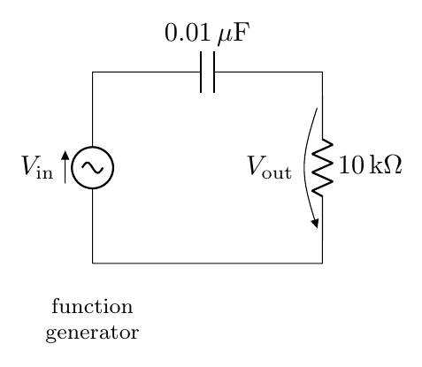
Sweep from 100 Hz to 10 kHz using the arrow keys and control knob on the generator to get a feel for the shape, then find the cutoff the same way. These are the same \(R\) and the same \(C\), so the measured cutoff should land on the same frequency you found in Part 4 — that agreement is the cleanest self-check in the lab.

Frequency	Input amplitude (V_pp)	Output amplitude (V_pp)	Phase difference (°)	Gain
? kHz				0.707

What type of filter is this now?
What is its measured cutoff frequency?

Note that these are the same two components — only the output node changed. That is the by-inspection test from Objective 2.4: ask what survives at DC.

Part 6 — Measure the Real Components (handout STEP 21)#

Take the components out of the breadboard and measure them with the ZLCR meter.

Measured \(R\): ______
Measured \(C\): ______

Recalculate the cutoff using the measured values. Is this closer to what you observed?

Why the numbers disagree

A ±10% capacitor moves the cutoff by roughly ±10% on its own, and the scope probe and breadboard add stray capacitance of their own. A disagreement you can explain is a good result. One you cannot explain means keep looking.

Part 7 — Hypothesize, Then Measure (handout STEP 22–26)#

Now build and investigate a third filter circuit — the one drawn on page 5 of the handout. Before you build it, look at it and hypothesize which type of filter it is (LPF, HPF, BPF, BSF/BRF), and write that hypothesis down. (Band-stop and band-reject are two names for the same filter; the handout writes BRF.)

Filter type (your hypothesis): ______________

Hypothesize first, then let the bench settle it

This circuit carries both an inductor and a capacitor, which makes it second-order — past the single-reactive-element R-C and R-L filters Objective 2.4 asks you to analyze. You are not expected to derive its response from scratch. Reason from what you do know — what a capacitor and an inductor each do at DC, and what each does at very high frequency — commit to an answer, and then measure. Whether the bench confirms your hypothesis or corrects it, the comparison is the learning; a hypothesis you had to revise is worth as much as one you did not.

As we did before, you will prototype the circuit and confirm the hypothesis by applying various input frequencies and measuring the input and output amplitudes with the oscilloscope.

Build the circuit on your breadboard, using the mini-grabber cable to connect from the function generator to the breadboard:

C = 0.01 µF — the same capacitor you have been using
L = 500 mH — the new inductor
\(R_{\text{out}} = 10\ \text{k}\Omega\) — the output resistor, with the output taken across it
\(R_L\) is the inductor’s internal resistance. The handout draws it inside a dashed box with the inductor because it is genuinely there in a real inductor — it does not need to be separately added to your breadboard.

Connect the input voltage to CH1 and the output resistor voltage to CH2.

Using the control knob on the function generator, sweep through 100 Hz to 10 kHz, keeping the input at 10 V_pp — the peak-gain judgment below only works if the input is held fixed. Estimate approximately where the peak gain occurs — the handout notes this value should fall between 1 and 5 kHz.

Frequency for peak gain: ______________

You will find that the gain at the “center frequency” is not quite equal to 1, because of the inductor’s internal resistance. Use the frequency that gets you closest to 1 as your center frequency.

Were you able to confirm your filter analysis hypothesis? ______________

If you have extra time, find the cutoff frequencies of this filter and estimate its bandwidth. Otherwise, power off and put away all equipment — you can leave the circuit components on top of the breadboard.

Good Lab Practice#

Keep the function generator’s output off while you change the circuit.
Check every connection before turning the output back on.
Analyze first — compute what you expect, so you notice immediately when a measurement disagrees.
Keep food and drink away from the equipment.

Files#

Handout — ECE215_AnalogFilterLab.pdf

Table of Contents