
Objective 2.2 — Ideal Filters#
LO# |
Description |
|---|---|
2.2 |
I can identify types of ideal filters, determine their cutoff frequencies, and analyze their output given an input sinusoidal signal or signal spectrum. |
By the end of this reading you should be able to:
Identify the four ideal filter types and what each passes.
Determine a filter’s cutoff frequency or frequencies.
Predict the output spectrum for a given input and filter.
Write the filtered signal back in the time domain.
Motivation#
Now that we understand analyzing a time-domain signal in the frequency domain, we can look at ideal filters. Ideal filters operate in the frequency domain and can help us keep and remove certain parts of a signal. For example, if you wanted to add more bass and less treble to a song, you would use an equalizer. In essence, an equalizer is a simple filter – one that lets us select which frequencies to keep and which to remove. (A real equalizer can also boost a band; the ideal filters in this course only pass or remove.) If you wanted more bass, then you could reduce the volume of the high frequencies while keeping the volume of the low frequencies the same. In this lesson, we will look at signals in the frequency domain and learn the basic functions of filters.
Key Concept
An ideal filter does not attenuate: each input spike either survives at full height or vanishes entirely. Real filters roll off gradually, which is Objective 2.4.
Electronic Filters#
The bandwidth of a signal drives our information processing and transmission systems. We will often reduce the bandwidth of our signals using a device known as an electronic filter which only allows certain frequencies to pass through the device and rejects all of the other frequencies. While we need to be careful in how we do this (because we can drastically change the original signal if we do too much filtering), it can help us communicate information faster, by reducing the size of the signal we need to process and transmit.
The telephone is a good example of what happens to a signal when a signal is filtered too much. When we speak on the phone, our voice is converted into a signal limited to a bandwidth of 4 kHz, even though human voices commonly include frequencies greater than 10 kHz. The phone companies figured out the lower 4 kHz of your voice is enough to understand what is being said and even recognize the voice of the speaker. This meant they could save bandwidth by filtering out those higher frequencies. However, since those high frequencies are missing, we can clearly tell the difference between someone speaking to us in person and when that same someone speaks to us over the phone.
There are four basic types of ideal electronic filters:
Low Pass Filters (LPF) which only allow frequencies below a specific cutoff frequency (fc) to pass
High Pass Filters (HPF) which only allow frequencies above a specific cutoff frequency (fc) to pass
Band Pass Filters (BPF) which only allow frequencies between two specific cutoff frequencies (fc1 and fc2) to pass
Band Stop Filters (BSF), also called band-reject filters (BRF), which block frequencies strictly between two specific cutoff frequencies (a component exactly at either cutoff passes) (fc1 and fc2). Both names are used, including on assessments.
A filter’s cutoff frequency is written \(f_{cutoff}\) on the equation sheet. In this course we shorten that to \(f_c\) when a filter has one cutoff, and \(f_{c1}\) and \(f_{c2}\) when it has two — the notation the quizzes use. Some of the figures below were drawn with older labels (\(f_{c/o}\), \(f_{cutoff,1}\), \(f_L\), \(f_H\)); they mean the same thing.
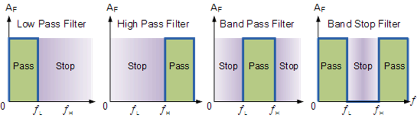
Figure 5: The four basic types of filters. This figure marks the cutoffs \(f_L\) and \(f_H\); read them as \(f_c\) on the low-pass and high-pass panels and as \(f_{c1}\), \(f_{c2}\) on the band-pass and band-stop panels. A low-pass filter and a high-pass filter each have only one cutoff, so on those two panels only the label at the drawn transition means anything — and do not confuse \(f_L\) / \(f_H\) here with the \(f_{low}\) / \(f_{high}\) of a signal in \(BW = f_{high} - f_{low}\).
For the purposes of this course, you may assume the ideal filter does not change the amplitude or phase of the input, and that every frequency outside the pass range is eliminated. The cutoff itself is inclusive: a component sitting exactly at a cutoff frequency passes, so a low-pass filter passes everything with \(f \leq f_c\) and a high-pass filter everything with \(f \geq f_c\) — the same non-strict convention the course uses later for Nyquist, \(f_s \geq 2f_{high}\). Returning to the telephone example, telephone companies use a LPF with a cutoff of 4 kHz to eliminate the upper frequencies in your voice and limit the amount of bandwidth they must transmit to 4 kHz.
Example Problem 1#
Design a filter system for a stereo to allow only high frequency signals (≥ 1.5 kHz) to be sent to the tweeter and only low frequency signals (≤ 1.5 kHz) to be sent to the woofer.
Understand: Tweeters are speakers designed to reproduce high frequency sounds, while woofers are speakers designed to reproduce low frequency sounds.
Identify Key Information:
Knowns: The frequency around which we want to split our signal is 1.5 kHz.
Unknowns: The filter type and the cutoff frequency
Assumptions: None
Plan: We want to divide our music signal into two pieces. We can do this by using two filters in parallel:
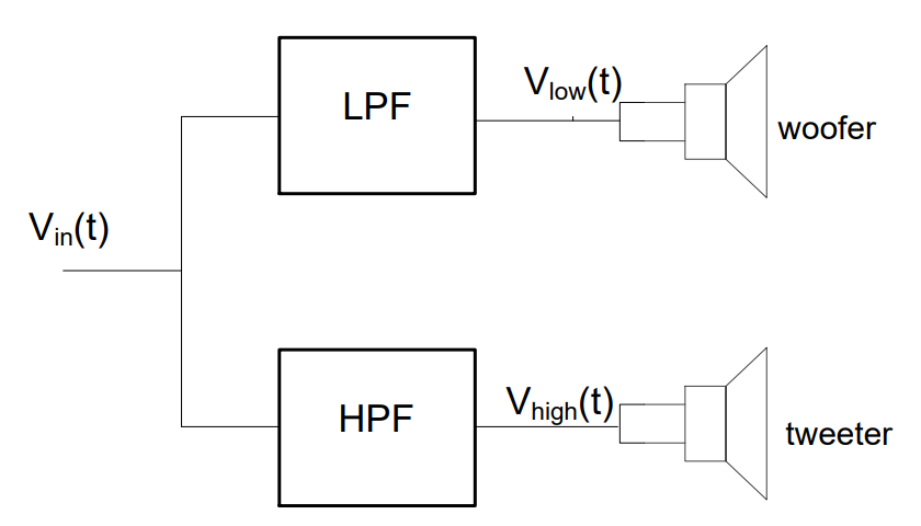
Figure 6: Two filters in parallel split one signal into two bands
The low pass filter (LPF) is used to feed the woofer, since it blocks the high frequencies and allows low frequencies to pass. Likewise, we use the high pass filter (HPF) to feed the tweeter, since it passes the high frequencies and blocks the low.
Solve: Since the problem specifies a cross-over frequency of 1.5 kHz, we simply choose filters with cutoff frequencies of 1.5 kHz. The following filter system can be used to feed the woofer and tweeter:
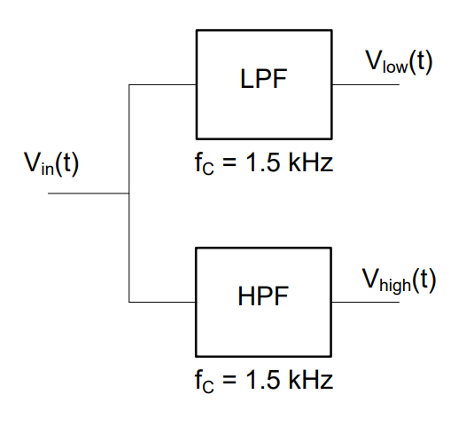
Figure 7: The finished crossover — both filters with a 1.5 kHz cutoff
Example Problem 2#
A signal passes through a band pass filter (BPF). What is the output signal?
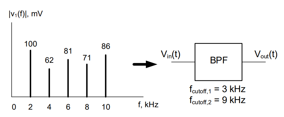
Figure 8: The input amplitude spectrum, with the band-pass cutoffs marked
Understand: The BPF eliminates frequencies outside the depicted cutoff frequencies and allows the frequencies within the band to pass.
Identify Key Information:
Knowns: The two cutoff frequencies and the BPF. We also know the input signal.
Unknowns: The output signal.
Assumptions: The BPF passes the band from 3 kHz to 9 kHz inclusive, and eliminates everything outside it.
Plan: Plot the cutoff frequencies and eliminate frequencies outside of that band.
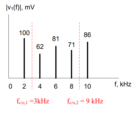
Figure 9: The input spectrum with the two cutoff frequencies drawn on it
Solve: The output signal from the depicted band pass filter is shown in the frequency spectrum graph below:
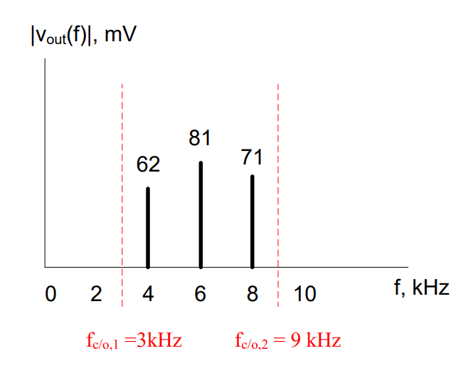
Figure 10: The output spectrum — the survivors keep their input heights
Type-along
The input is \(v_{in}(t) = 4 + 6\cos(2\pi\cdot 500t) + 3\cos(2\pi\cdot 2000t) + 5\cos(2\pi\cdot 8000t)\).
Find the output of a low-pass filter with \(f_c = 1\) kHz.
Find the output of a high-pass filter with \(f_c = 1\) kHz.
Find the output of a band-pass filter from 1 kHz to 5 kHz.
Solution
The input spikes sit at 0 Hz, 500 Hz, 2 kHz, and 8 kHz.
1. Survivors below 1 kHz: DC and 500 Hz. \(v_{out} = 4 + 6\cos(2\pi\cdot 500t)\).
2. Survivors above 1 kHz: 2 kHz and 8 kHz. The DC term is removed. \(v_{out} = 3\cos(2\pi\cdot 2000t) + 5\cos(2\pi\cdot 8000t)\).
3. Only 2 kHz falls inside the band. \(v_{out} = 3\cos(2\pi\cdot 2000t)\).
Wrap-Up#
There are four ideal filter types — low-pass, high-pass, band-pass, and band-stop — and each is defined by one or two cutoff frequencies. To find an output, go spike by spike and ask whether each falls in the passband or the stopband. Note that a high-pass filter always removes DC, which is exactly how a demodulator strips a bias in Block 3.
Objective 2.3 gives you the tool for building real filters: modeling capacitors and inductors as complex resistors.