
Objective 2.6 — Signal Conditioning#
LO# |
Description |
|---|---|
2.6 |
I can implement signal conditioning to avoid aliasing and clipping and to ensure maximum compatibility of the dynamic ranges between two devices. |
By the end of this reading you should be able to:
Explain the three pitfalls: aliasing, clipping, and wasted dynamic range.
Specify an anti-aliasing filter.
Compute the gain \(K\) and bias \(B\) that map a transducer onto an ADC’s range.
Verify that the conditioned signal uses the full range without clipping.
Transducers and Signal Conditioning#
Introduction#
In previous lessons, we discussed a number of basic electrical components that are used in all kinds of useful circuits for myriad applications. In this lesson, we will continue to build on that foundation to understand how devices use electrical signals to communicate with one another. But first, we need to discuss how we initially get an electrical signal that we would want to communicate somewhere else. This is where transducers come into play.
Take your computer mouse and move it around a little bit and see what happens. If your computer is actually turned on while you do this, you will probably see the pointer on your computer display move left or right or up or down in sync with the movements you made with the mouse.
Now think about what is really happening during this process. If you have an optical mouse, the light from a light-emitting diode (LED) reflects off of the surface of your desk and is picked up by an opto-electronic sensor which sends the image to an image-processing chip. This chip compares the image from one moment to the next and determines how much the mouse has moved and in what direction. The mouse then creates an electronic signal that contains this movement information and sends it to the computer, which, in turn, processes that signal and causes the mouse cursor to move with respect to the rest of the display. The following block diagram succinctly captures the process:

Up to this point, we’ve only studied signals related to the transmission and flow of power. While these signals are certainly useful, electrical signals can also be used to transmit and process signals conveying information. The Air Force spends a massive amount of time gathering information with its satellites, reconnaissance aircraft, and unmanned aerial systems (UAS) but the data is worthless if we can’t get it to the right place for our people to use it.
Transducers#
Transducers are devices that interface the physical world with the electrical world. We will consider two primary types of transducers: input transducers and output transducers. Input transducers convert a physical signal into an electrical signal. For example, a microphone turns sound waves into electrical signals. This conversion is useful if we want to process the vocal signal digitally, or if we want to transmit this signal over a network. In fact, any sensor we want to analyze using a computer must include an input transducer. Figure 1 shows an example of physical information translated into electrical data where a voice has been converted into a voltage waveform.
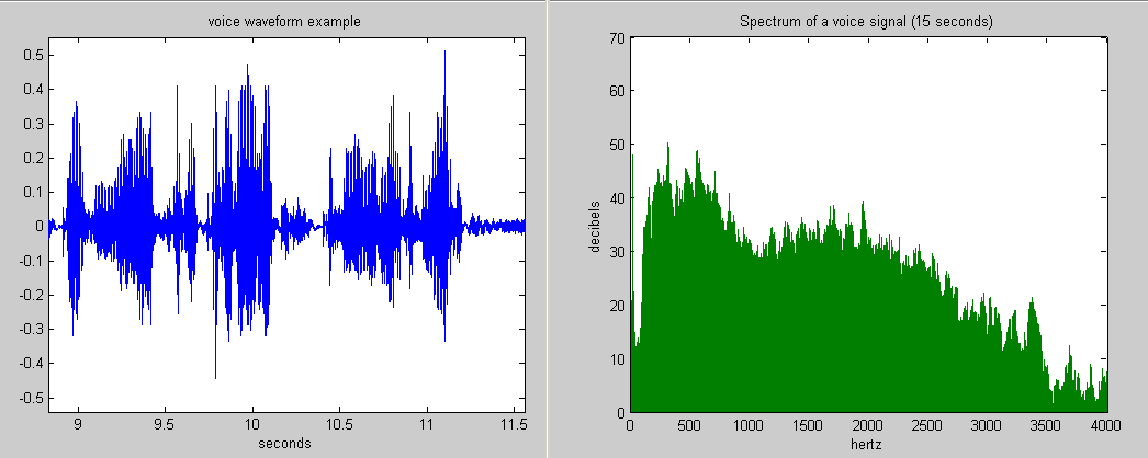
Figure 1: Example of voice converted to an electrical signal
http://www.answers.com/topic/frequency-spectrum
Conversely, output transducers convert an electrical signal into a physical signal. In keeping with the transmission of your voice over a communications network – someone will likely want to hear what you said, so they might have headphones connected to their receiving radio. In this case, the headphones are converting the electrical signal back to sound waves again; therefore, the speakers are an example of an output transducer.
Three Pitfalls Between a Transducer and an ADC#
Before we build anything, it is worth naming the three ways the connection between a transducer and a converter goes wrong. Conditioning exists to fix all three, and every one of them destroys information at the instant of conversion — which is why the fix has to sit before the ADC.
Aliasing (a frequency problem). A transducer picks up more than you asked for: noise, interference, and signal content above the band you care about. Objective 2.5 showed that anything above \(f_s/2\) comes back as an alias, and that no processing afterward can separate it from the real signal. The fix is a low-pass anti-aliasing filter ahead of the converter.
Specifying that filter takes two steps. First, set the cutoff just above the highest frequency you actually want: with the R-C low-pass of Objective 2.4, \(f_{cutoff} = 1/(2\pi RC)\), so choosing \(f_{cutoff}\) chooses \(R\) and \(C\). Then pick the sampling rate from that cutoff, \(f_s \geq 2 f_{cutoff}\) — and leave margin above it. A first-order R-C is still passing \(0.707\) of the signal at its own cutoff and rolls off only 20 dB per decade, so sampling at exactly \(2 f_{cutoff}\) folds the surviving content right back into your band. Oversampling to a few times \(2 f_{cutoff}\) is what makes a real filter behave like the ideal one on the slide.
Clipping (the signal is too big). If the conditioned signal ever leaves the range \([V_{min}, V_{max}]\), the converter saturates: it reports its extreme code and nothing more. The peaks of the waveform come out flattened, which both destroys the peak values and creates frequency content that was never in the original signal. Like aliasing, it cannot be undone afterward. Never let the conditioned signal exceed the converter’s range — not once, not at the peak.
Wasted dynamic range (the signal is too small). A device’s dynamic range is the span between its smallest and largest usable signal; for an ADC that is \(V_{max} - V_{min}\). This is the opposite failure, and it is easy to miss because nothing looks broken. A transducer swinging \(\pm 2\) V into an ADC spanning \(\pm 5\) V uses only 40% of the available range — 102 of the 256 levels of an 8-bit converter, about 6.7 effective bits out of the 8 you paid for. Every unused level is resolution thrown away.
The first pitfall is fixed with a filter. The other two are fixed with the gain and bias that the rest of this reading develops, and the goal is always the same: land the signal’s extremes exactly on the converter’s extremes.
Instrumentation and Signal Conditioning#
Most input transducers do not provide electrical signals that are powerful enough to be displayed. For example, the output of most microphones is in the millivolt range. In order for this signal to be useful, we have to do something to the signal. If we follow the analogy of the microphone further, we can’t drive a speaker (an output transducer) with the low voltage produced by a microphone. One way to condition a signal is to build an instrumentation system consisting of amplification and biasing.
Key Concept
Instrumentation connects input and output transducers in a meaningful way.
Key Concept
Conditioning is one linear map, \(v_{out} = K v_{in} + B\). Map min to min and max to max, subtract the two endpoint equations to eliminate \(B\) and solve for \(K\), then back-substitute — and always check both endpoints at the end.
Amplification and Biasing#
Amplification is a straightforward concept. An amplifier takes small values that we simply need to make larger and multiplies them by a constant value. If the dynamic range of the input and output transducers are symmetric around zero, amplification alone will suffice for signal conditioning. Oftentimes though, the dynamic range of either our input or output transducers is not symmetric around zero and, when we amplify our signal, we find the magnitude of our values is correct, but they are offset from where we need them to be. In this case, we can add a bias voltage to shift the output appropriately. The device we use to add two voltages together is known as a summer. The generic flow for any instrumentation is shown in Figure 2.
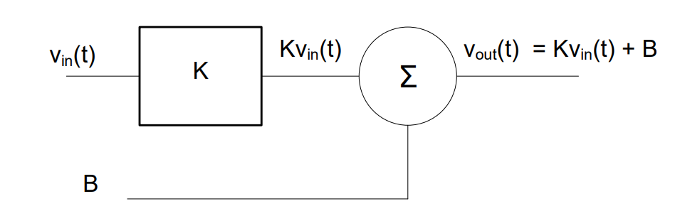
Figure 2: Block diagram for a generic instrumentation system.
In this flow, we see that the input and output are related by the equation:
So, the input voltage is first multiplied by the constant K, which is a gain factor. The DC bias B is then added to the result of that operation. Practically, this allows us a great deal of flexibility when designing instrumentation to interface various input and output transducers. In general, input transducers will correlate a physically expected behavior with a voltage. A thermocouple, for example, is an input transducer that senses a temperature and outputs a voltage for that specific temperature. However, we may want to use another device, such as a temperature gauge (which is an output transducer) to view the output of the thermocouple. In most cases, the temperature gauge expects a different range of voltages, which it will then correlate to a temperature display. Using the gain and bias of the instrumentation system, we can translate the actual output range of the thermocouple to the expected input range of the temperature gauge. Let’s look at an example problem to see how this plays out in a real world scenario.
Example Problem 1:#
A small aircraft uses an input transducer called a thermocouple to measure the outside air temperature. When the temperature is -60° C, the thermocouple produces -2 mV. When the temperature is 50° C, it produces 8 mV. The signal from the thermocouple is used by a temperature gauge in the cockpit to display the outside air temperature to the pilot. The gauge requires -5 V to display a temperature of -60° C and 10 V to display 50° C. Design the interface to connect these two devices (assuming both the thermocouple and gauge are linear devices).
Understand: The pilot wants to know the outside air temperature, which is sensed by the thermocouple and displayed by the temperature gauge. However, the thermocouple produces very low voltages, while the gauge requires much larger voltages. We need something to convert the relatively small thermocouple voltage into the correspondingly higher gauge voltage, so we can display the correct temperature. Obviously, the signal needs to be amplified, because we’re going from mV to V. Unfortunately, converting -2 mV into -5 V and also converting 8 mV into 10 V with a single constant gain amplifier is not possible. Therefore, we will need to take advantage of both our gain and bias.
Identify Key Information:
Knowns: We know the correlation between temperature and voltage for the thermocouple and for the temperature gauge.
Condition |
vin(t), Thermocouple Input |
vout(t), Gauge Input |
|---|---|---|
-60° C |
-2 mV |
-5 V |
50° C |
8 mV |
10 V |
Unknowns: We want to know the gain (K) and bias (B) of the instrumentation system.
Assumptions: The gain and the bias will be produced by linear devices, meaning the correlation between the input and output is always a straight line.
Plan:
To see the big picture, we plot the voltage produced by the thermocouple against the voltage required by the gauge:
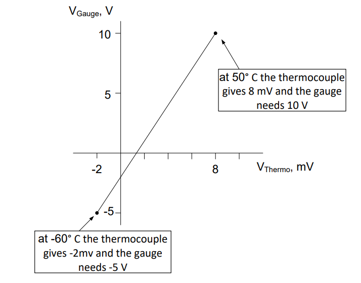
Since we assume the devices are linear, we can draw a straight line between them, to represent what we want our interface to do. As the thermocouple voltage rises linearly from -2 mV to 8 mV, we want the gauge voltage to rise from -5 V to 10 V.
Recall the straight-line equation in the slope-intercept form is y = mx + b, where m is the slope and b is the y-intercept. For a signal conditioning system that accounts for this shift in voltage, we use a very similar equation:
In this equation, K is the gain of a scalar multiplier and B is a DC bias voltage. The block diagram for this required signal conditioning is:
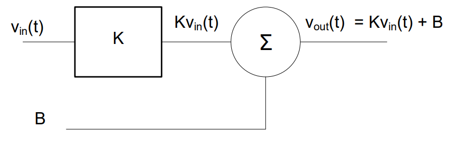
Here, we see the input voltage is multiplied by the amplifier gain, K. A bias voltage, \(B\), is then added to the result of that operation to produce the correct relationship for \(v_{out}\). Here, the circle with the Greek sigma inside is a summer, which is an electronic device that mathematically adds the two input signals. We will use the extreme cases of the thermocouple-gauge relationship to write two independent equations and solve for both K and B.
Solve: Let’s start by applying this generic block diagram to the system we want to design:
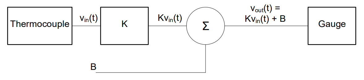
Now let’s look at the expected conditions and expected behaviors of the transducers we need to design this specific system. When the temperature is -60° C, the thermocouple produces -2mV, we will multiply this by K and then add B, and the result should be -5 V. Likewise, when the temperature is 50° C, the thermocouple produces 8 mV, we multiply this by K, add B , and the gauge should get 10 V. These are our two extreme cases, and they allow us to write two independent equations to solve for our two unknowns (K and B)
Plugging both sets of values into the equation for our line gives the following:
Since we have two equations with two unknowns, we can solve for both K and \(B\). There are several ways we can do this (your calculator should be able to do it using its built-in equation solver mode), but there is a simple approach which will work for all our signal conditioning problems. By subtracting the second equation from the first, we can quickly solve for K, since the B terms will cancel. Here’s what it looks like:
Solving for K gives:
As you can see, K is a dimensionless number with no units — because both sides of the equation are voltages. When the output of the map is not a voltage, K carries the ratio of the two units instead: in the Lesson 22 lab you will fit a distance in centimeters against a voltage, and there K comes out in cm·V. We can now plug K back into either equation to solve for B. If we use the first equation, we get:
Solving this for \(B\) gives:
Therefore, we need to build an interface that accomplishes the following function:
Answer: The design for an interface between the thermocouple and the gauge is as follows:
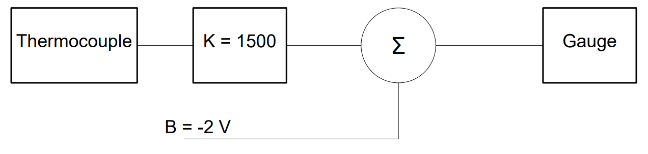
Example Problem 2:#
Using the system designed in the previous problem, what voltage would be sent to the gauge if the thermocouple produces 1.3 mV?
Understand: We must calculate the effect of our interface on a particular input signal received from the thermocouple.
Identify Key Information:
Knowns: We know the equation for our instrumentation and the input voltage.
Unknowns: We want to know the output of the instrumentation system, which is the input to the temperature gauge.
Assumptions: Our devices are all linear.
Plan: Plug the given input value into our instrumentation equation.
Solve: The equation for the system above is
Since vin(t) = 1.3 mV, we have:
Answer: This system would send -50 mV to the gauge if the thermocouple voltage was 1.3 mV.
Example Problem 3:#
An elevator actuator for a UAS requires 1 V to move the elevator fully down and -9 V to move the elevator fully up. The control unit produces -1 mV when fully down and 4 mV for fully up. Design the interface between the control unit and the actuator.
Understand: Since we are building an instrumentation as an interface for two transducers, we’ll solve this exactly like the earlier problem. The most important step in these problems is identifying which device is inputting into the interface and which device needs the output from the interface, as the inputs and outputs can be a bit confusing. In this case, the control unit is providing vin(t), while the elevator actuator needs vout(t).
Identify Key Information:
Knowns: We know the correlation between our expected physical behaviors and the voltages for both our input transducer (control unit) and the output transducer (actuator), as shown in the following table
Condition |
vin(t) – Input from Control Unit |
vout(t) – Output to Actuator |
|---|---|---|
Fully down |
-1 mV |
1 V |
Fully up |
4 mV |
-9 V |
Unknowns: We are trying to find the gain (K) and bias (B) for our instrumentation, which will interface between the control unit and the actuator.
Assumptions: Our devices are linear.
Plan: We will use the instrumentation equation and the extreme cases of the input/output (i/o) table above.
Solve: Using the values from the table above, we can build two equations:
If we subtract the bottom equation from the top equation, we get:
Using the first equation to solve for \(B\),
Answer: The required interface is as follows:
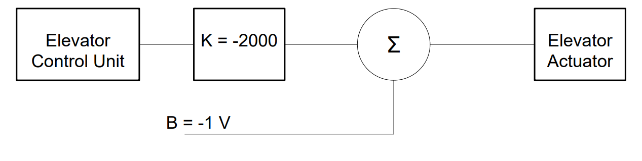
Type-along
A pressure sensor outputs \(0.5\) V at minimum pressure and \(4.5\) V at maximum. It feeds a 10-bit ADC with an input range of \(0\) V to \(3.3\) V. The signal has content up to \(200\) Hz.
Specify the anti-aliasing filter and a suitable sampling rate.
Find the gain \(K\) and bias \(B\) that use the ADC’s full range.
Verify both endpoints.
What would happen with no conditioning at all?
Solution
1. A low-pass filter with \(f_{cutoff}\) just above 200 Hz — say 250 Hz — then \(f_s \geq 500\) Hz. A practical choice is \(f_s = 1\) kHz for margin.
2. \(0 = K(0.5) + B\) and \(3.3 = K(4.5) + B\). Subtracting: \(-3.3 = -4K\), so \(K = 0.825\); then \(B = -0.4125\) V.
3. At \(4.5\) V: \(0.825(4.5) - 0.4125 = 3.3\) V. ✓ At \(0.5\) V: \(0.825(0.5) - 0.4125 = 0\) V. ✓
Note \(K < 1\) — this is attenuation plus a downward shift, not amplification. Conditioning does not always mean gain.
4. Everything above 3.3 V would clip (losing the top quarter of the sensor’s range), while the 0–0.5 V portion of the ADC would never be used. Both pitfalls at once.
Wrap-Up#
Three pitfalls sit between a transducer and an ADC: aliasing (a frequency problem, fixed with a low-pass filter), clipping (signal too big), and wasted dynamic range (signal too small). The last two are fixed with one linear map, \(v_{out} = K v_{in} + B\), found by mapping min to min and max to max. All of it must happen before the converter — afterward the information is already gone.
Objective 2.7 turns to what the computer does with the bits once it has them.