Objective 3.2 — Demodulation

LO#	Description
3.2	I can design a demodulator given a modulated signal for envelope and synchronous detection.

By the end of this reading you should be able to:

1. Compute the modulation efficiency of an AM signal.

2. Describe how an envelope detector works and when it is valid.

3. Describe how a synchronous detector works and why it always works.

4. Design either demodulator, specifying filter types and cutoff frequencies.

Demodulation Intro

This lesson focuses on demodulating the signals to recover the original information. We will also look at the different trade-offs that are made when choosing how to modulate and demodulate a signal.

Key Concept

\(\eta = \alpha^2/(\alpha^2 + 2)\). Only the sidebands carry the message, so at \(\alpha = 1\) — the best an envelope detector can handle — efficiency is just \(1/3\).

Modulation Efficiency

Previously, we introduced the concept of adding a bias signal to our message before sending the message through a function multiplier. We compared the waveforms and spectra for three different modulation indexes (using the same 2 V message tone, a carrier amplitude of A_c = 2 V, and biases of 0 V, 2 V, and 3 V, respectively), as shown below. The envelope is \(A_c[B + v_m(t)]\), so it peaks at \(A_c(B + A_m)\): 4 V, 8 V and 10 V. In the spectra, each sideband has height \(A_cA_m/2 = 2\) V and the carrier has height \(A_cB\): 0 V, 4 V and 6 V. You can see as we add more bias to our message, the envelopes of the time-domain waveform draw apart until they are completely separated for modulation indexes less than 1. At the same time, a frequency component appears in the spectrum at the carrier frequency that grows larger as we increase the amount of bias added. The signals on the far left and far right are examples of two classes of amplitude modulation:

• Double sideband, suppressed carrier (DSB-SC): Information is carried in sidebands found on either side of the carrier signal. Signal power is split evenly between the two sidebands.

• Double sideband, large carrier (DSB-LC): Information is carried in sidebands found on either side of the carrier signal. Signal power is split between the two sidebands AND the carrier frequency.

These two names are used only in this reading. The slides and the equation sheet describe the same two cases as no carrier (no bias, \(B = 0\)) and carrier present (a bias was added).

Over-modulated	Fully modulated (100%)	Under-modulated
α → ∞	α = 1	α = 0.667

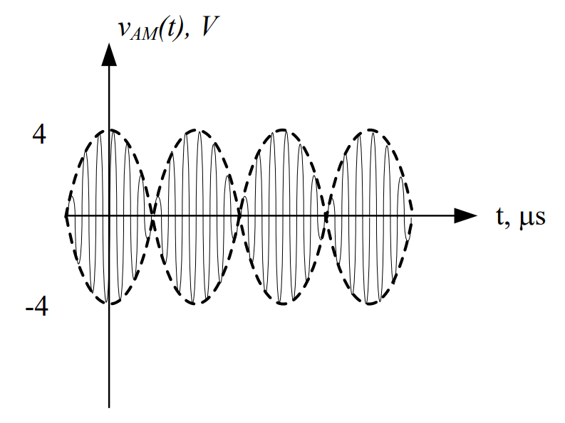
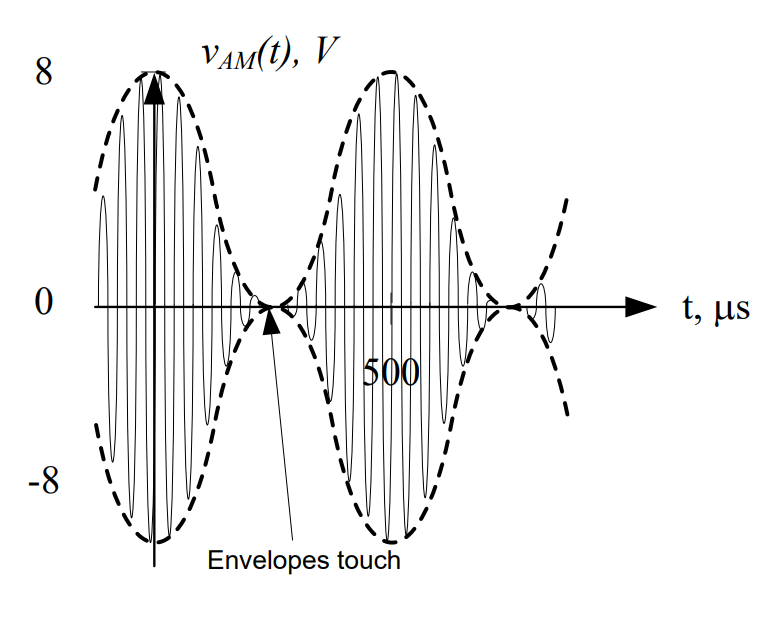
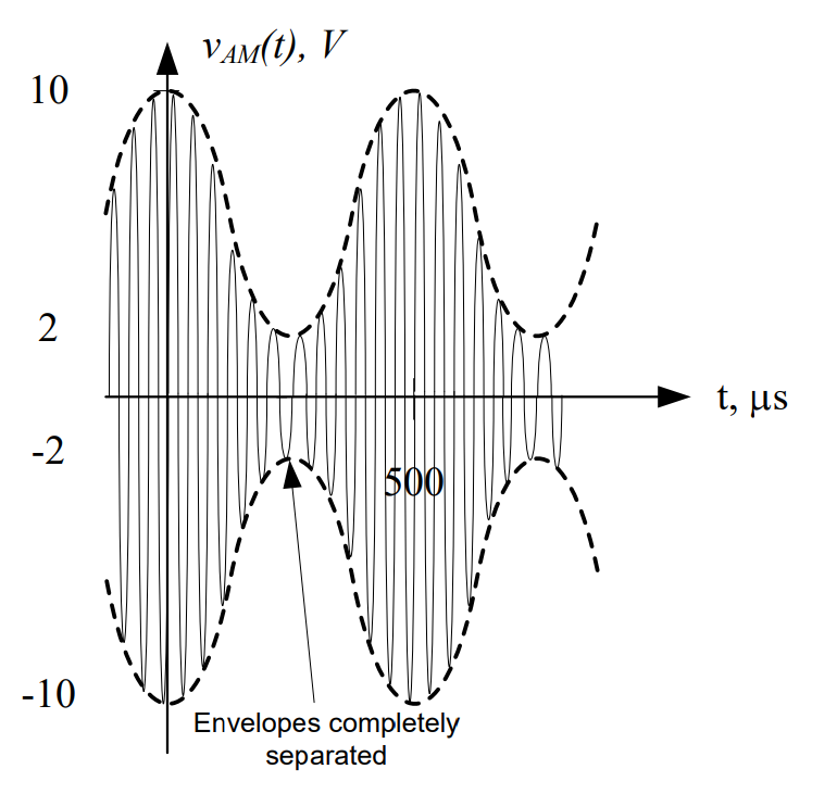
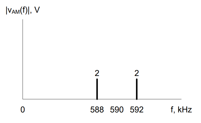
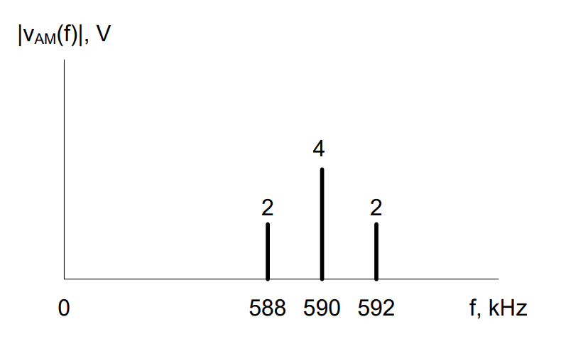
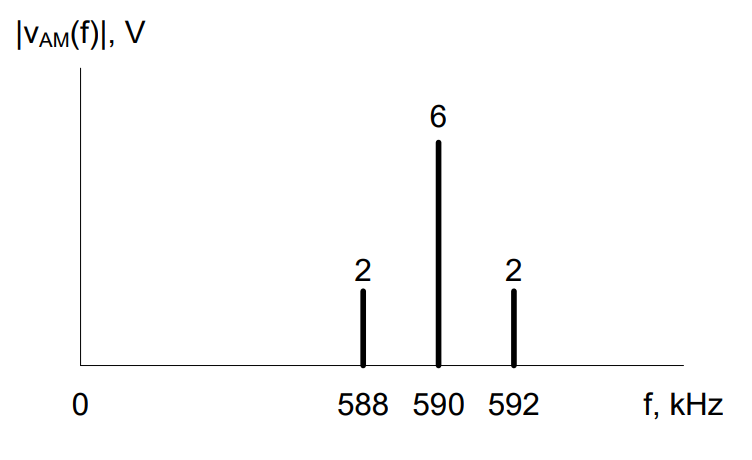
In order to calculate the efficiency of AM, we need to identify what part of the signal is useful power and what part is “wasted” power. As we can see above, the sidebands hold our original information (and are therefore “useful”) while the component at the carrier frequency is simply there because we pumped more power into our AM signal by adding a bias. When we speak of the efficiency of amplitude modulation, η, we are referring to the ratio of the power transmitted in the sidebands to the total power transmitted in the AM signal. Note η is always defined in terms of power, not voltage - be careful! We can calculate η directly from the known power values by:

\[\eta = \frac{\text{useful power}}{\text{useful power} + \text{wasted power}} = \frac{\text{upper sideband power} + \text{lower sideband power}}{\text{total power}}\]

Recall power can be calculated by squaring the RMS voltage and dividing by the resistance \(\left( P = \frac{V_{rms}^{2}}{R} \right)\). Since the RMS voltage of a sinusoid is simply its amplitude divided by \(\sqrt{2}\), its power can be expressed as \(P = \frac{A^{2}}{2R}\), where \(A\) is the sinusoid’s amplitude. To simplify our power calculations, we often normalize resistance, which means we set \(R = 1\ \Omega\). If we apply this principle and use the relationship \(\alpha = \frac{A_{m}}{B}\) — the single-tone case of \(\alpha = \max(\text{message})/B\) — we can derive a simple equation for AM efficiency:

\[\eta = \frac{\alpha^{2}}{\alpha^{2} + 2}\]

While the original equation for efficiency is valid for any type of message signal, this simplified equation is only valid for a message that consists of a single sinusoid. This type of sinusoidal “message” is called a test tone by radio engineers and is most commonly heard when the federal Emergency Alert System is tested. It is the form on the equation sheet, so we will use the simple equation to calculate AM efficiency in this course, as an estimate whenever the message is not a single tone.

Note the efficiency of DSB-SC is always 100% (do you know why?). When the bias is 0 V, \(\alpha = \infty\), and \(\eta\) becomes 1, or 100%. If you add a bias, \(\alpha\) becomes finite. For the fully modulated (100%) case, \(\alpha = 1\), and \(\eta\) becomes 0.33, or equivalently 33%. This means 67% of the transmitted power is wasted in the carrier frequency component! So why do most AM radio stations opt to use DSB-LC for their signals? Well, it comes down to what kind of demodulator you want to use to retrieve your message.

Demodulation – Envelope Detector

Consider an under-modulated AM signal again. The message signal has enough bias that the signal entering the function multiplier is completely positive. This means that the resulting AM signal has completely separate envelopes, thus the original message can be easily retrieved if we can isolate the upper envelope.

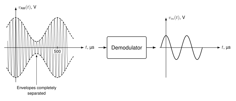
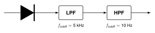
The device that accomplishes these tasks is called an envelope detector. An envelope detector consists of a diode, a low pass filter, and a high pass filter. Recall from Objective 1.7 (AC-to-DC conversion) that a diode is simply an electronic component that acts as a “one-way street” for current. The diode used in an envelope detector allows just the positive part of the signal to pass through it. Therefore, as an AM signal, v_AM(t), arrives at the input to the diode, the diode blocks the negative portion of the AM signal, resulting in the signal v_R(t). v_R(t) carries only the envelope on the positive portion of the carrier. This process is called rectification.

v_R(t), which contains both high and low frequency components in its spectrum, is filtered through the low pass filter, which results in a signal that has the same shape as the positive envelope of v_R(t), but contains a DC offset due to the bias of the original signal. Finally, the high pass filter is used to eliminate the component of the low pass filtered version of v_R(t) which has a frequency of 0 Hz (this corresponds to the original bias, \(B\)). The final result is a signal which replicates the original message signal, v_m(t). These signal processing steps are shown pictorially below.

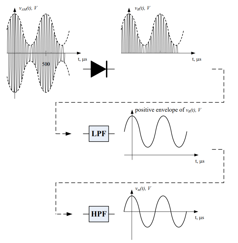
Since diodes, capacitors, and resistors are very cheap, demodulators can be inexpensive if the signal is fully modulated or under-modulated. In fact, during WWII, GIs were able to build the radio below (which is basically an envelope detector) from on-hand parts. We sacrifice efficiency in order to gain a cheap solution to recovering our information.

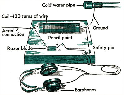
A foxhole radio: the razor blade and pencil point act as the diode. Image: Wired GeekDad, 2009.

Example Problem 1

A voice message is input into an AM modulator. The output of the modulator is shown below. Design an AM demodulator to recover the message signal.

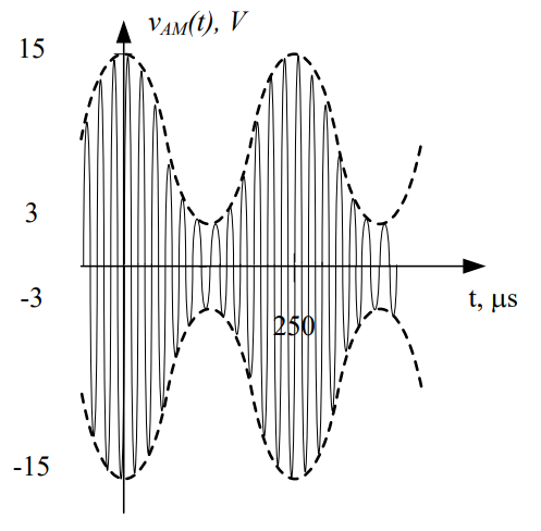
Understand: Here, we have an under-modulated signal, which means we can use an envelope detector. The message we want to recover is the upper envelope (dashed line) in the graph above. To do this, we need to remove the negative portion of the signal, the high frequency carrier signal, and the bias.

Identify Key Information:

• Knowns: We know the signal is under-modulated, and we know the period of the message signal (250 µs).

• Unknowns: We don’t know the frequency or period of the carrier signal.

• Assumptions: None.

Plan: Since the signal is under-modulated, we can use an envelope detector. Since we know the form of an envelope detector, we only need to define the cutoff frequencies of the LPF and HPF.

Solve: Feeding the under-modulated signal into the diode results in the following waveform:

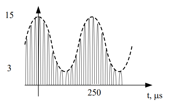
In order to remove the high frequency carrier signal, we need to pass this signal through a low pass filter, but we don’t have the cutoff frequency. In the end, we want to keep the envelope, but remove the higher frequencies. Therefore, we can set the cutoff frequency of the LPF just above that of the message envelope. The frequency of the original message was:

\[f_{m} = \frac{1}{T} = \frac{1}{250\ \mu\text{s}} = 4\ \text{kHz}\]

So the cutoff frequency must be at least 4 kHz, to keep the envelope, and below the AM signal’s own band around the carrier, to remove the high frequency information. We are not told the carrier frequency here, which is one reason the habit in this course is to choose a cutoff just above the message; 5 kHz will do. The result is:

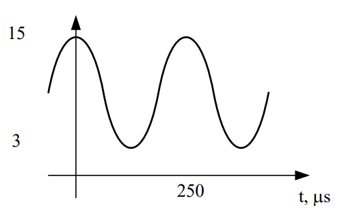
(The plot shows the shape of the low pass filter’s output. Its height depends on the circuit: an ideal rectifier followed by an ideal low pass filter returns the envelope scaled by \(1/\pi\), while a diode-and-capacitor detector follows the peaks, as drawn.)

The last step is to remove the bias signal from the message. This step doesn’t require any calculations because we already know the frequency of a bias signal (0 Hz). Since it’s always 0 Hz, we simply need a high pass filter with a cutoff greater than 0 Hz and no higher than the lowest frequency in the message; 10 Hz will suffice.

Answer: The envelope detector below will successfully retrieve our original voice message.

Before we move on, let’s quickly review what the three components in an envelope detector do:

• Diode: Kills the negative voltages

• Low pass filter: Kills the carrier

• High pass filter: Kills the bias

Also, we have two important rules:

• The cutoff frequency of the low pass filter must be at least the highest frequency in the message, \(f_{\text{cutoff}} \ge f_{m,\max}\), and below the AM signal’s own band, which starts at \(f_c - f_{m,\max}\). Any cutoff in that window works; the habit in this course is to choose one just above \(f_{m,\max}\).

• The cutoff frequency of the high pass filter will always be slightly greater than 0 Hz (nominally 10 Hz).

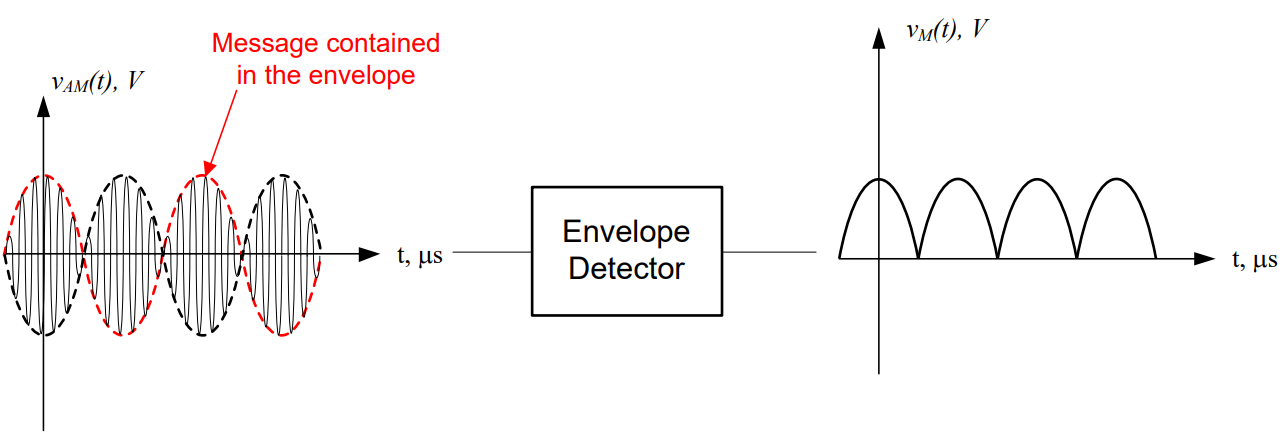
And the most important concept of all - envelope detectors DO NOT work for over-modulated signals, or DSB-SC modulation. They simply trace the upper envelope, and as you can see by the example below, they definitely give you the wrong message back.

Key Concept

A design names every block and every value: LPF cutoff just above \(f_{m,\max}\), HPF cutoff at about 10 Hz, and for synchronous detection, a local oscillator at exactly \(f_c\) with a stated amplitude \(A_{\text{LO}}\).

Demodulation – Synchronous Detector

If we have an over-modulated signal, then we have to use a more complicated demodulator. Demodulation is still fairly straightforward, but requires more than simple circuit components. Synchronous demodulation is the opposite of modulation – the incoming signal is mixed (using a function multiplier) with a sinusoid at the original carrier frequency, and the output is run through a series of filters. The receiver generates that sinusoid itself, with a local oscillator.

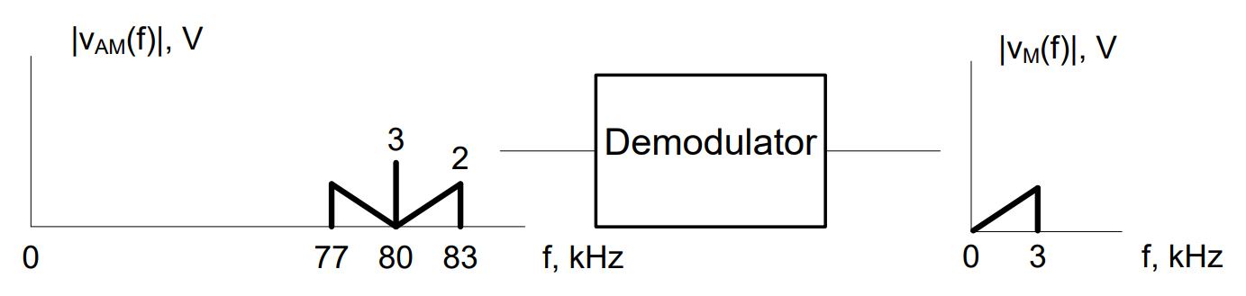
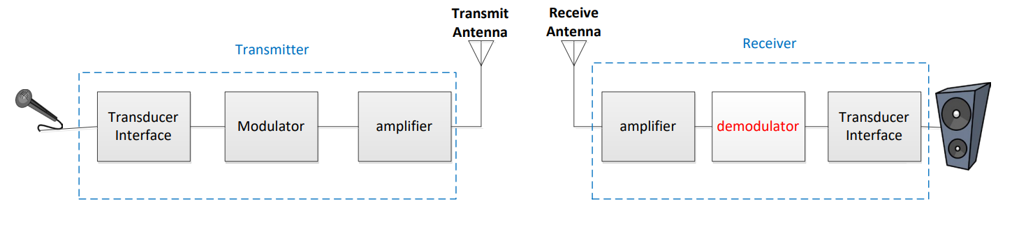
Figure 1: Block diagram for a demodulator.

The block diagram of a synchronous demodulator, which works for all modulated signals, is:

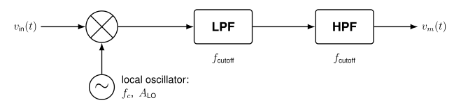
Figure 2: Block diagram for a synchronous detector.

This reading writes the local oscillator’s frequency as \(f_c\), since it must equal the carrier frequency, and its amplitude as \(A_{\text{LO}}\), so that \(A_c\) keeps meaning the transmitter’s carrier amplitude. A quiz or exam may still call it “the carrier signal amplitude, \(A_c\)”: that means this demodulating carrier, the oscillator in the detector, not the transmitter’s.

Consider the modulated signal shown in Figure 1. First, we need to shift the 80 kHz modulated signal back down to baseband (0 Hz) and then we need to eliminate the bias term. This is the crucial point to designing a synchronous detector – determining what signal to multiply the AM signal by, which allows recovery of the message. We will again use the properties of the function multiplier.

Let’s start by looking at the AM signal itself:

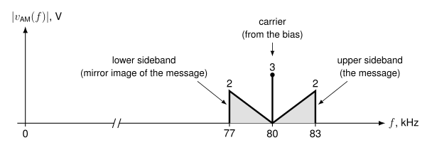
As shown in the above graph, the signal is a combination of the upper sideband, the carrier (which is there because a bias was added), and the lower sideband.

In an AM signal, a center spike (if present) will always be located at the carrier frequency. Therefore, we can easily tell from this graph that the carrier signal was 80 kHz. We can also tell the original message was located from 0 to 3 kHz. We can shift the signal using a function multiplier and a local oscillator with a frequency of 80 kHz and an amplitude of \(A_{\text{LO}}\) = 2 V. This results in two key actions:

• The signal will be shifted up by 80 kHz (the sum of the demodulating frequency and the original frequency). Instead of being centered at 80 kHz, it is now centered at 160 kHz (80 kHz + 80 kHz).

• The signal will also be shifted down by 80 kHz (the difference of the demodulating frequency and the original frequency).

• Note: each shifted copy has \(A_{\text{LO}}/2\) times the height of the original, the same factor of one half as in modulation. The amplitudes stay the same here only because we are conveniently using \(A_{\text{LO}}\) = 2 V, so \(A_{\text{LO}}/2 = 1\).

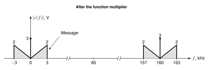
Notice that the message signal, represented by a triangle, is exactly where we want it to be.

However, we see there are “negative frequencies” here and, as we know, negative frequencies don’t exist. They come straight from the difference rule: the lower sideband at 77 kHz lands at 77 − 80 = −3 kHz. Because \(\cos(-x) = \cos(x)\), a component at −3 kHz is the same sinusoid as one at +3 kHz, so the portion of the signal that is shown between 0 and −3 kHz folds over and is added to the message between 0 and 3 kHz. This doubles the message (2 V + 2 V = 4 V at 3 kHz), but not the spike at 0 Hz, which landed there only once:

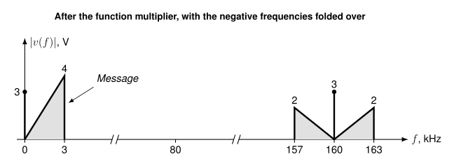
In general, if the transmitter used a carrier amplitude \(A_c\) and a bias \(B\), a message tone of amplitude \(A_m\) arrives as two sidebands of height \(A_cA_m/2\) and a carrier of height \(A_cB\). After the function multiplier the two sidebands add at baseband and the carrier becomes a DC term:

\[\text{recovered tone} = 2 \cdot \frac{A_{\text{LO}}}{2} \cdot \frac{A_cA_m}{2} = \frac{A_cA_{\text{LO}}A_m}{2} \qquad\qquad \text{DC term} = \frac{A_cA_{\text{LO}}B}{2}\]

Notice we still have a bias signal and a higher frequency component to remove. Therefore, after passing through the function multiplier, we send the signal through a low pass filter. Just as we did with the envelope detector, we set the cutoff frequency of the low pass filter to be at least the highest frequency in the message signal (which, for this case, is 3 kHz) and below the lowest unwanted component, the image that starts at 157 kHz. Any cutoff in that window works; following the habit in this course, we choose \(f_{\text{cutoff}}\) = 4 kHz. This results in:

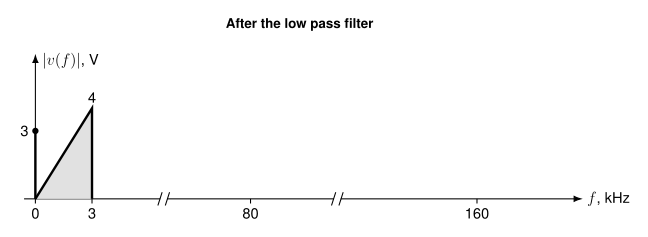
Now all that remains is to remove the bias. Just as with the envelope detector, the bias can be removed by passing the signal through a high pass filter with \(f_{\text{cutoff}}\) > 0 Hz. In this case, we’ll use 10 Hz again. This returns us to our original message signal, scaled by \(A_cA_{\text{LO}}/2\): the recovered spectrum peaks at 4 V, which is the original message’s own peak only if the transmitter’s \(A_c\) was 1 V.

The final form of the synchronous detector is:

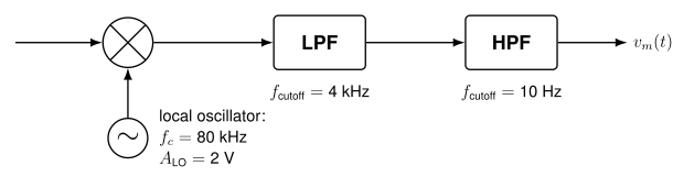
In summary, the three components in a synchronous detector:

• Function multiplier: Moves the AM signal back down to baseband frequencies

• Low pass filter: Removes the high frequency image added by the function multiplier

• High pass filter: Removes the bias

The design rules for these components are:

• The frequency of the demodulating signal (the local oscillator), which is passed to the function multiplier, should be equal to the carrier frequency of the original modulated signal. State its amplitude, \(A_{\text{LO}}\), as well

• The cutoff frequency of the low pass filter will always be greater than or equal to the highest frequency in the message, and below the lowest unwanted component: the image, which starts at \(2f_c - f_{m,\max}\). The habit in this course is to choose it just above \(f_{m,\max}\)

• The cutoff frequency of the high pass filter will always be slightly greater than 0 Hz (nominally 10 Hz)

If other channels share the band (frequency division multiplexing, Objective 3.1), a band pass filter that passes \(f_c - f_{m,\max}\) to \(f_c + f_{m,\max}\) can be placed ahead of either detector to select the wanted channel. An envelope detector needs it. A synchronous detector can do without it, but the function multiplier also shifts a neighboring channel at carrier \(f_n\) down to \(|f_n - f_c|\), so the low pass filter’s cutoff must then stay below that neighbor’s lowest shifted frequency.

Type-along

A received AM signal has a carrier at \(f_c = 80\) kHz and message content up to \(12\) kHz. The envelope swings between \(2\) V and \(14\) V.

1. Taking \(A_c = 1\), find the bias \(B\) and \(\max(\text{message})\).

2. Find \(\alpha\) and classify the signal.

3. Find the modulation efficiency.

4. Design a demodulator.

Solution

1. The envelope is \(A_c[B + v_m(t)]\), so with \(A_c = 1\) its maximum is \(B + \max(\text{message}) = 14\) and its minimum is \(B - \max(\text{message}) = 2\). Adding and subtracting gives \(B = 8\) V and \(\max(\text{message}) = 6\) V.

2. \(\alpha = 6/8 = 0.75\), so under-modulated. The envelope limits give the same answer without \(A_c\): \(\alpha = (\max - \min)/(\max + \min) = 12/16 = 0.75\).

3. \(\eta = 0.75^2/(0.75^2 + 2) = 0.5625/2.5625 = 22.0\%\).

4. Either detector works since \(\alpha \le 1\). The cheap choice is an envelope detector: rectifier → LPF with a cutoff of 15 kHz (just above \(f_{m,\max}\); anything from 12 kHz to below \(80 - 12 = 68\) kHz works) → HPF with a cutoff of 10 Hz. A synchronous detector would use a local oscillator at 80 kHz with the same two filters.

Wrap-Up

Only the sidebands carry information, so \(\eta = \alpha^2/(\alpha^2+2)\). An envelope detector is cheap but needs \(\alpha \le 1\); a synchronous detector works on anything but must know \(f_c\) exactly in frequency and phase. Its function multiplier scales every component by \(A_{\text{LO}}/2\) and shifts it by \(f_c\), so the two sidebands add at baseband and the carrier becomes a DC term for the high pass filter to remove. Broadcast under-modulates deliberately — wasting transmit power to make millions of receivers cheap is the right trade.

Objective 3.3 turns to how the signal gets off the wire and into the air.