23. Text Vectorization#
The first step in Natural Language Processing is to get the words into a format that we can do math on them.
23.1. Pre-reading#
Objectives#
Use stop words to make text more signifigant.
Vectorize text to enable machine learning.
23.2. Stop Words#
For this example we will use Inaugural Addresses from American Presidents.
Go to the website now and think how you might put all of these into an easy-to-ingest document.
Fortunately, I’ve already extracted some of these and placed them in a CSV located in this folder on GitHub.
Explore Data#
As always, we should preview some stats about what we are diving in to.
Prompt GPT4-Advanced Data Analytics: Use pandas to provide a quick summary of this CSV
import pandas as pd

# Path to 'inaugural_addresses.csv'
csv_path = "inaugural_addresses.csv"

# Load the CSV into a pandas DataFrame
df = pd.read_csv(csv_path)

# Display the first few rows of the DataFrame and its summary
df_head = df.head()
df_info = df.info()

df_head
Word Clouds#
Unlike numerical data, we cannot easily do things like mean, median, or standard deviation with text data.
Let’s try a word cloud, just for fun.
%pip install wordcloud
import matplotlib.pyplot as plt
from wordcloud import WordCloud

# Set up the figure size and number of subplots
fig, axes = plt.subplots(nrows=df.shape[0], ncols=1, figsize=(15, 30))

# Loop through each row of the DataFrame and generate a word cloud
for i, (index, row) in enumerate(df.iterrows()):
    # Create a word cloud object
    wc = WordCloud(
        background_color="white", stopwords=[], max_words=100, width=800, height=400
    )

    # Generate the word cloud from the 'Text' column
    wc.generate(row["Text"])

    # Display the word cloud on the subplot
    axes[i].imshow(wc, interpolation="bilinear")
    axes[i].axis("off")
    axes[i].set_title(f"{row['President']} ({row['Year']})", fontsize=37)

# Adjust layout
plt.tight_layout()
plt.show()
Stop Words#
Hmm, that isn’t very helpful! Fortunately, there are multiple lists of English Stop Words in Python.
In fact, wordcloud.STOPWORDS is an option!
# TODO: Re-produce word clouds with wordcloud.STOPWORDS
Lemmatization#
Another common text pre-processing technique is lemmatization.
In linguistics, is the process of grouping together the inflected forms of a word so they can be analyzed as a single item, identified by the word’s lemma, or dictionary form.
Stemming reduces an inflected word to its base; for example: runs; running; ran –> “run”.
Lemmatizing goes further by using knowledge of surrounding words.
The word “better” has “good” as its lemma. This link is missed by stemming, as it requires a dictionary look-up.
The word “walk” is the base form for the word “walking”, and hence this is matched in both stemming and lemmatization.
The word “meeting” can be either the base form of a noun or a form of a verb (“to meet”) depending on the context; e.g., “in our last meeting” or “We are meeting again tomorrow”. Unlike stemming, lemmatization attempts to select the correct lemma depending on the context.
Optional Exercise#
Re-create the inaugural address word clouds after lemmatization.
23.3. Text Vectorization#
Important
Delete and restart your kernel to clear out the previous runs.
Let’s use Kagggle’s Twitter US Airline Sentiment dataset.
First, read the Data Card. What month and year are these from? How were they collected? What transformations have been done?
Import and explore data#
Yes, always the first step.
import pandas as pd

# TODO: Explore the data
Stemming#
Let’s apply stopwords and stemming to our tweets.
%pip install nltk
import nltk

# Download the resources from nltk
nltk.download("punkt")
nltk.download("stopwords")
import nltk
from nltk.corpus import stopwords
from nltk.stem import PorterStemmer
from sklearn.feature_extraction.text import CountVectorizer

# Initialize the stemmer
stemmer = PorterStemmer()


# Define a function that applies stemming and stopwords removal
def preprocess(text):
    # Tokenize the text
    tokens = nltk.word_tokenize(text)

    # Remove stopwords and apply stemming
    tokens = [
        stemmer.stem(word)
        for word in tokens
        if word.lower() not in stopwords.words("english")
    ]

    return " ".join(tokens)


# Apply the function to the "text" column
df["processed_text"] = df["text"].apply(preprocess)

# Preview the result
print(df["text"].head())
print(df["processed_text"].head())
Bag of Words#
The naive - but sometimes highly effective - approach is the “Bag of Words” approach.
Simply count how many times words show up!
Start with the train/test split.
from sklearn.model_selection import train_test_split

# Splitting the data into training and testing sets
X = df["processed_text"]
y = df["airline_sentiment"]
X_train, X_test, y_train, y_test = train_test_split(
    X, y, test_size=0.2, random_state=42
)

X_train.shape, X_test.shape
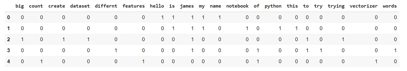
CountVectorizer#
Convert a collection of text documents to a matrix of token counts.
See Medium: Basics of CountVectorizer
from sklearn.feature_extraction.text import CountVectorizer
from sklearn.linear_model import LogisticRegression
from sklearn.pipeline import make_pipeline
from sklearn.metrics import accuracy_score

# Create a pipeline that first transforms the text data into a bag-of-words representation
# and then trains a logistic regression classifier
pipeline = make_pipeline(CountVectorizer(), LogisticRegression(max_iter=1000))

# Train the classifier
pipeline.fit(X_train, y_train)

# Predict on the test set
y_pred = pipeline.predict(X_test)

# Calculate the accuracy
accuracy = accuracy_score(y_test, y_pred)
accuracy