Block 1 — Introduction, Frames, and Errors

By the end of this block you should be able to:

1. Explain what a navigation system estimates.

2. Distinguish between truth, measurement, and estimate.

3. Identify the five reference frames used in this course: ECEF, NED, RTN, Aircraft Body, Spacecraft Body.

4. Use a Direction Cosine Matrix (DCM) to move a vector or a point between frames.

5. Define position error and reduce it to horizontal (\(e_H\)) and vertical (\(e_V\)) operational metrics.

6. Explain why frame consistency must be established before any statistics or integrity logic is applied.

What is Navigation?

A navigation system estimates the state of a vehicle relative to a chosen reference frame. The state vector typically contains position, velocity, and attitude:

\[\begin{split} \hat{\mathbf{x}} = \begin{bmatrix} \text{position} \\ \text{velocity} \\ \text{attitude} \end{bmatrix}. \end{split}\]

Every element of the state is the output of a process that fuses imperfect inputs. Sensors carry noise and bias, the dynamic models we propagate forward in time are simplifications, and the assumptions baked into the algorithms (linearization points, model orders, numerical tolerances) introduce additional error. A useful navigation solution is therefore the pair

\[ (\hat{\mathbf{x}},\ \mathbf{P}), \]

where \(\mathbf{P}\) is the state error covariance that quantifies how much we trust each component of \(\hat{\mathbf{x}}\). Guidance, control, mission effectiveness, and safety all depend on having both the estimate and an honest measure of its uncertainty.

Key Concept

A navigation solution is not a point. It is a state estimate paired with an uncertainty. Reporting one without the other hides the most important information.

Truth, Measurement, and Estimate

Three quantities show up in every navigation analysis. Keep them straight.

Symbol	Name	What it represents
\(\mathbf{x}_{\text{truth}}\)	Truth	The actual state of the vehicle. We never know this exactly; in test we approximate it with a higher-grade reference.
\(\mathbf{z} = f(\mathbf{x}) + \mathbf{v}\)	Measurement	What a sensor outputs. It is some (often nonlinear) function of the truth, corrupted by noise \(\mathbf{v}\).
\(\hat{\mathbf{x}}\)	Estimate	What the navigation system reports.

The estimation error is

\[ \mathbf{e} = \hat{\mathbf{x}} - \mathbf{x}_{\text{truth}}. \]

In flight test we evaluate a navigation system by collecting many samples of \(\mathbf{e}\) over a representative trajectory and asking whether the resulting empirical distribution meets requirements. That is the entire game.

Why Frames Matter

Suppose someone hands you error = [2, 1, -0.5] and asks whether it meets a 5 m horizontal targeting requirement. Before you can answer you must ask:

• In what frame? ECEF? NED? Body?

• What units? Meters? Feet? Radians?

• Where is the origin or the reference point?

Without that context the numbers are not interpretable, and any statistic computed from them is meaningless.

Key Concept

Navigation computations only make sense when every quantity is expressed in a known, consistent frame with known units and a known origin.

Reference Frames

We use five reference frames in this course. Three describe where the vehicle is in the world (ECEF, NED, RTN), and two describe where things are on the vehicle itself (aircraft body, spacecraft body). The first three are “world” frames; the last two are “platform” frames that rotate with the vehicle.

ECEF — Earth-Centered, Earth-Fixed

ECEF is a global Cartesian frame attached to the rotating Earth. Its origin sits at the Earth’s center of mass and its axes are:

• \(X\): toward the intersection of the equator and the prime meridian (latitude \(0^\circ\), longitude \(0^\circ\)).

• \(Y\): toward the equator at longitude \(90^\circ\)E.

• \(Z\): along the Earth’s spin axis, toward the North Pole.

ECEF is the natural frame for GNSS satellite geometry and global trajectories because it covers the whole Earth without singularities. It is much less intuitive when you want to reason about local error metrics like “how far off were we to the north?”.

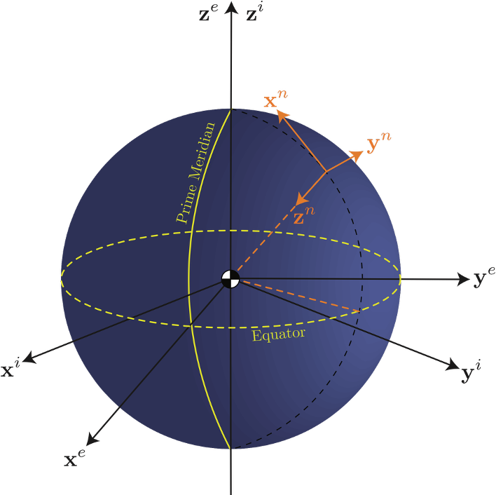
Fig. 1.1. The ECEF frame: origin at Earth’s center, \(X\) through (lat 0°, lon 0°), \(Z\) through the North Pole.

NED — Local-Level North-East-Down

NED is a tangent-plane frame defined at a chosen reference latitude/longitude/height. Its axes are:

• \(N\): north along the local meridian.

• \(E\): east along the local parallel.

• \(D\): down, normal to the local-level plane.

NED assumes the surface is locally flat near the reference point. That assumption is excellent over the few-kilometer scales typical of a single test point, and it is what makes NED the standard frame for aviation navigation reports. Position errors, velocity errors, and covariance ellipses all become operationally interpretable in NED.

RTN — Radial-Transverse-Normal (the spacecraft NED)

For spacecraft in orbit there is no “down” in the gravity-vector sense, but there is still a natural local frame defined by the orbit geometry. The Radial-Transverse-Normal (RTN) frame is centered on the spacecraft and oriented to its instantaneous position and velocity vectors:

• \(R\): radial, outward from Earth’s center along the spacecraft’s position vector.

• \(T\): along-track, tangent to the orbit in the direction of motion.

• \(N\): cross-track, normal to the orbital plane (right-hand rule).

RTN rotates with the orbit, so it has a time-varying angular rate. For a circular orbit at altitude \(h\), the angular rate is just the orbital mean motion. RTN is the standard frame for orbital relative motion: it underlies Clohessy-Wiltshire (Hill’s) equations for rendezvous and proximity operations, and any time you see a “radial / along-track / cross-track” decomposition of an orbital error, the underlying frame is RTN.

The mental picture: RTN is to a spacecraft what NED is to an aircraft — both are local-level frames that follow the vehicle along its curved reference path.

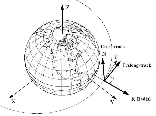
Fig. 1.2. The RTN frame: \(R\) outward from Earth’s center along the spacecraft’s position vector, \(T\) along-track in the direction of motion, \(N\) cross-track normal to the orbital plane.

Aircraft Body Frame (b-frame, FRD)

The aircraft body frame is rigidly attached to the airframe. The convention used in this course is forward-right-down (FRD):

• \(X\): forward along the nose.

• \(Y\): out the right wing.

• \(Z\): down through the belly.

Body is the frame in which sensors actually measure. An accelerometer feels specific force along its case axes, which are nominally aligned to the body frame. A gyroscope measures angular rate of the body relative to an inertial frame. Inertial mechanization equations work in body frame and then rotate the result into NED for reporting.

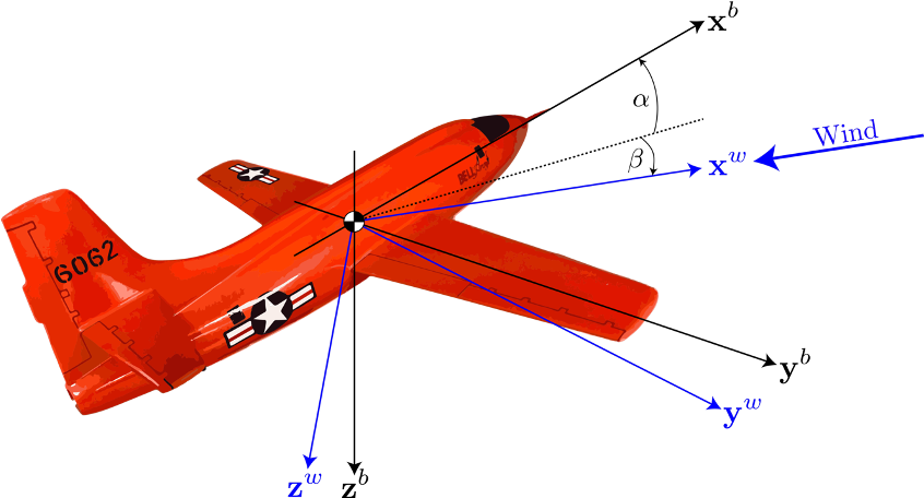
Fig. 1.3. The aircraft body frame is rigidly attached to the vehicle. \(X\) forward, \(Y\) out the right wing, \(Z\) down.

Spacecraft Body Frame (sc-frame)

The spacecraft body frame plays the same role as the aircraft body frame, but with axis conventions driven by the satellite’s mission rather than aerodynamics. Origin sits at the spacecraft center of mass (or the principal-inertia reference point). Axes are mission-dependent:

• \(X\): usually aligned with the primary instrument boresight or a nadir-pointing direction.

• \(Y\): along a solar array, side panel, or other structural reference.

• \(Z\): completes the right-hand rule.

The spacecraft body frame is the reference for star trackers, gyros, sun sensors, and thrusters, and is the working frame for attitude determination, attitude control, and pointing analysis. To express the spacecraft state in a world frame, you transform body-frame vectors into RTN or directly into ECI via the spacecraft attitude.

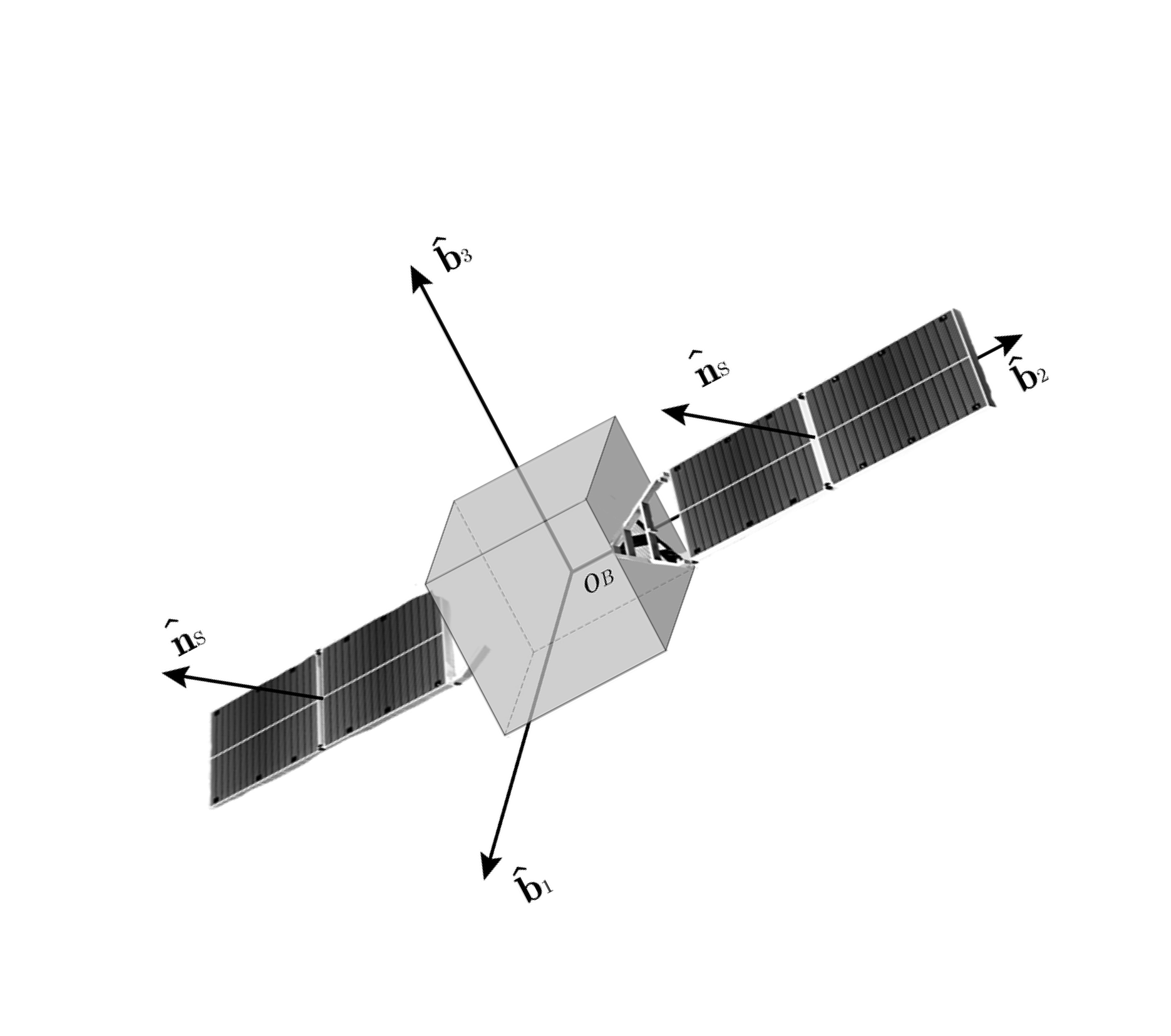
Fig. 1.4. The spacecraft body frame is rigidly attached to the spacecraft structure. Specific axis assignments are mission-dependent: typical conventions point \(X\) along the primary instrument boresight or toward nadir, \(Y\) along a solar array, with \(Z\) completing the right-hand rule.

The aircraft body frame and the spacecraft body frame are conceptually identical: each is a vehicle-fixed sensor reference. The axis labels just track different mission conventions.

Frame Transformations: Direction Cosine Matrices

A Direction Cosine Matrix (DCM) takes the components of a vector in one frame and returns the components of the same physical vector in a different frame. The notation used in this course is

\[ \mathbf{v}^b = \mathbf{C}_a^b\, \mathbf{v}^a, \]

where \(\mathbf{C}_a^b\) rotates components from frame \(a\) to frame \(b\).

DCMs are orthonormal, which has two consequences worth memorizing:

\[ \mathbf{C}^\top \mathbf{C} = \mathbf{I}, \qquad \left(\mathbf{C}_a^b\right)^{-1} = \left(\mathbf{C}_a^b\right)^{\top} = \mathbf{C}_b^a. \]

The inverse equals the transpose. If you have \(\mathbf{C}_a^b\) and want to go the other way, you transpose, you do not invert.

Key Concept

A DCM rotates components, not the physical vector. Same arrow in space, different numerical representation.

2D DCM Example

For two coplanar frames separated by an angle \(\theta\), the DCM is

\[\begin{split} \mathbf{C}_a^b(\theta) = \begin{bmatrix} \cos\theta & \sin\theta \\ -\sin\theta & \cos\theta \end{bmatrix}. \end{split}\]

Apply it to a vector and the components change while the vector itself stays put. The 2D DCM demo in this block (linked from the sidebar) lets you sweep \(\theta\) continuously or step through a teaching sequence, watch both the input components \(\mathbf{v}^a\) and the rotated components \(\mathbf{v}^b\) update at every step, and confirm visually that the norm \(\lVert\mathbf{v}\rVert\) is preserved up to floating-point round-off — the numerical fingerprint of orthonormality. A MATLAB implementation is also included at code/DcmExample.m.

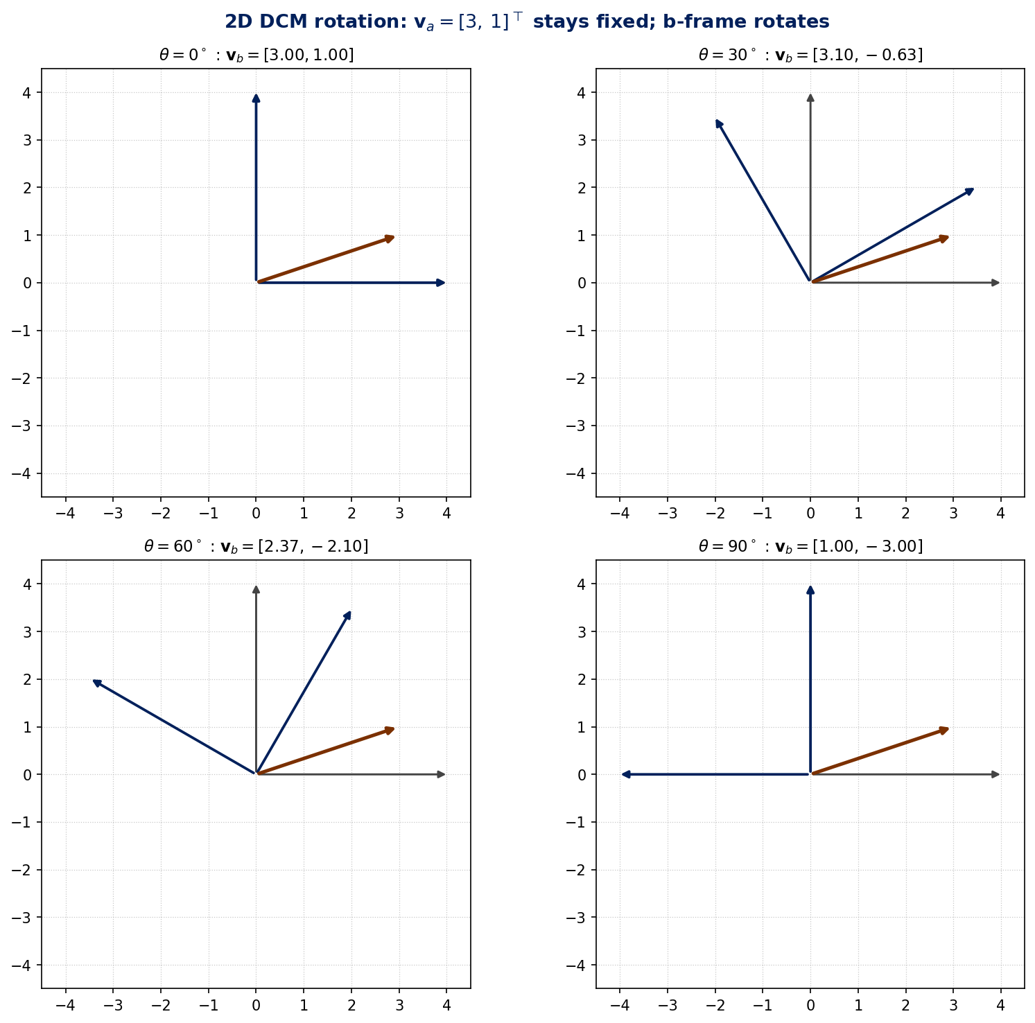
Fig. 1.5. Snapshots of the 2D DCM rotation at \(\theta = 0°, 30°, 60°, 90°\). The brown arrow (the physical vector \(\mathbf{v}\)) does not move. Only the blue b-frame axes rotate. The components \(\mathbf{v}^b\) change accordingly while \(\lVert\mathbf{v}\rVert\) is preserved. Open the interactive demo in the sidebar to sweep \(\theta\) continuously.

3D DCMs and Moving Points

In three dimensions, \(\mathbf{C}_a^b \in \mathbb{R}^{3\times 3}\) and the rule is the same:

\[ \mathbf{v}^b = \mathbf{C}_a^b\, \mathbf{v}^a. \]

One common parameterization is the Roll-Pitch-Yaw (Euler 321) sequence:

\[ \mathbf{C}_a^b(\phi, \theta, \psi) = \mathbf{R}_z(\psi)\, \mathbf{R}_y(\theta)\, \mathbf{R}_x(\phi). \]

The order matters. Yaw, then pitch, then roll is not the same as roll, then pitch, then yaw. Quaternions avoid this pitfall and avoid gimbal lock at \(\theta = \pm 90^\circ\), but for reporting and ground analysis RPY remains common because the angles are operationally meaningful.

A subtlety that catches people: rotating a vector between frames uses the DCM alone, but rotating a point also requires a translation, because points are tied to a specific origin. If \(\mathbf{r}_{a\rightarrow b}\) is the position of frame \(b\)’s origin expressed in frame \(a\), then

\[ \mathbf{p}^b = \mathbf{C}_a^b \left(\mathbf{p}^a - \mathbf{r}_{a\rightarrow b}\right). \]

For LLH-to-ECEF-to-NED chains the translation comes from the chosen reference point. Pick the reference deliberately and document it in your reports.

Error Definitions in NED

Once everything is expressed in a consistent frame, the error vector is just a subtraction:

\[\begin{split} \mathbf{e}_{\text{NED}} = \hat{\mathbf{p}}_{\text{NED}} - \mathbf{p}_{\text{NED, truth}} = \begin{bmatrix} e_N \\ e_E \\ e_D \end{bmatrix}. \end{split}\]

Two scalar metrics show up in nearly every test report:

\[ e_H = \sqrt{e_N^2 + e_E^2}, \qquad e_V = \lvert e_D \rvert. \]

\(e_H\) is horizontal miss distance. \(e_V\) is vertical miss. Most accuracy requirements are stated as the upper 95% confidence bound on these two scalars, with a minimum effective sample size to make the statistic credible. We will define \(N_\text{eff}\) in Block 9.

Quick Exercise

Given

\[\begin{split} \mathbf{p}_{\text{truth}} = \begin{bmatrix} 1000 \\ 500 \\ -50 \end{bmatrix} \text{ m}, \qquad \hat{\mathbf{p}} = \begin{bmatrix} 1003 \\ 498 \\ -49 \end{bmatrix} \text{ m}, \end{split}\]

compute \(\mathbf{e}_{\text{NED}}\), \(e_H\), and \(e_V\). Then ask: if you rotated the entire problem into ECEF, what numerical quantities would change? What would not?

Solution

\(\mathbf{e}_{\text{NED}} = \hat{\mathbf{p}} - \mathbf{p}_{\text{truth}} = [+3,\ -2,\ +1]^\top\) m.

\(e_H = \sqrt{3^2 + (-2)^2} = \sqrt{13} \approx 3.61\) m.

\(e_V = |+1| = 1\) m.

If you rotated into ECEF, the components of \(\mathbf{e}\) would change (the same physical error vector now expressed in different axes), but the magnitude \(\lVert \mathbf{e} \rVert\) would not. The split into “horizontal” and “vertical”, however, only makes sense in NED, because horizontal-versus-vertical is defined by the local-level plane.

Target Location Error: A Worked Example

Block 1’s second demo, Target Location Error (TLE), takes you through the full LLH → ECEF → NED chain on a realistic targeting scenario. A truth target location near Edwards AFB is converted to ECEF, a sensor estimate with a small lat / lon / height offset is converted to ECEF, and both are projected into a local-level NED frame centered at the truth point. The demo reports \(e_N\), \(e_E\), \(e_D\), and the operational metrics \(e_H\) and \(e_V\), and includes a latitude experiment that exposes the cos(latitude) effect: the same arcsecond of longitude error becomes very different metric error depending on where on Earth the scenario is.

Open the demo from the sidebar to set up your own truth / sensor pair, drag the sensor pin in the NE plot, and watch the conversion chain update live. A MATLAB implementation is also included at code/TargetLocationError.m, with the LLH↔ECEF and ECEF↔NED utilities in code/navutils/.

Wrap-Up

Navigation estimates a vehicle’s state relative to a chosen reference frame and reports it together with an uncertainty \(\mathbf{P}\). Truth, measurement, and estimate are distinct quantities, and the estimation error is \(\mathbf{e} = \hat{\mathbf{x}} - \mathbf{x}_{\text{truth}}\). Five frames carry the load: ECEF (global Cartesian), NED (local tangent plane for aircraft), RTN (local-orbit plane for spacecraft), aircraft body (vehicle-fixed FRD), and spacecraft body (vehicle-fixed mission-dependent). DCMs move vectors between frames; points additionally require a translation. Position error reduces to two operational scalars, \(e_H\) and \(e_V\), and frame consistency is the prerequisite for every statistic and every integrity computation that comes later.

The next block looks at where those position errors come from in the first place: small inertial sensor errors, integrated through the mechanization equations, become growing drift.