Block 5 — Multi-State Kalman Filter for Navigation

By the end of this block you should be able to:

1. Explain why navigation problems require multi-state estimation.

2. Generalize the scalar Kalman filter equations to vector states.

3. Write the state transition matrix \(\mathbf{F}\) for constant-velocity 2D motion.

4. Write the measurement matrix \(\mathbf{H}\) for a position-only sensor.

5. Interpret the off-diagonal terms of the covariance matrix \(\mathbf{P}\) as cross-correlation between states.

6. Run a 4-state filter that simultaneously estimates 2D position and velocity from noisy 2D position fixes.

Why Multiple States?

The scalar filter in Block 4 estimated a single quantity. Real navigation systems have to estimate many quantities simultaneously:

• 3D position and 3D velocity.

• 3-axis attitude (or its small-angle linearization).

• Sensor biases on accelerometers and gyroscopes.

• Receiver clock errors when GPS is in the loop.

A modern operational INS/GPS filter typically carries 12 to 20 states. The math does not change: it is still predict-then-update, still inverse-variance fusion. But every scalar becomes a vector, every variance becomes a covariance matrix, and every formula learns to respect matrix order.

Key Concept

The Kalman filter scales from one state to many by replacing scalars with vectors and variances with covariance matrices. The conceptual machinery — predict, fuse with measurement using the optimal weight, repeat — is unchanged.

A 4-State Tracking Problem

The cleanest non-trivial example: a vehicle moving in 2D with approximately constant velocity, observed by a noisy 2D position sensor. The state vector contains 2D position and 2D velocity:

\[\begin{split} \mathbf{x}_k = \begin{bmatrix} p_{x,k} \\ p_{y,k} \\ v_{x,k} \\ v_{y,k} \end{bmatrix}. \end{split}\]

State transition matrix

For constant-velocity motion, position evolves as \(p_{k+1} = p_k + v_k\,\Delta t\) and velocity stays the same. Stacked as a matrix:

\[\begin{split} \mathbf{x}_{k+1} = \mathbf{F}\,\mathbf{x}_k, \qquad \mathbf{F} = \begin{bmatrix} 1 & 0 & \Delta t & 0 \\ 0 & 1 & 0 & \Delta t \\ 0 & 0 & 1 & 0 \\ 0 & 0 & 0 & 1 \end{bmatrix}. \end{split}\]

The off-diagonal \(\Delta t\) entries are what couple velocity into position. They are the structural reason that a velocity measurement can tighten the position estimate through the cross-covariance, and equivalently the reason that a position-only sensor still produces a good velocity estimate after a few cycles. The filter learns velocity from the rate of change of position because that information is built into \(\mathbf{F}\).

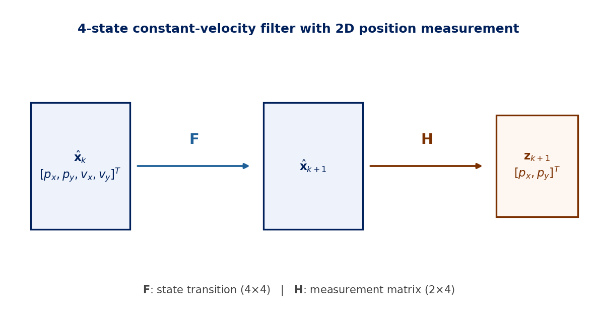
Fig. 1.1. The 4-state filter propagates the state with \(\mathbf{F}\) and projects to the measurement space with \(\mathbf{H}\). Both matrices are \(4\times 4\) and \(2\times 4\) respectively for this example.

Process noise

Real motion is not perfectly constant-velocity. Unknown accelerations along each axis inject uncertainty into all four states (acceleration affects velocity directly and position by integration). The standard model treats the unknown acceleration as zero-mean white noise with variance \(\sigma_a^2\). Working through the integrals:

\[\begin{split} \mathbf{Q} = \sigma_a^2 \begin{bmatrix} \dfrac{\Delta t^4}{4} & 0 & \dfrac{\Delta t^3}{2} & 0 \\ 0 & \dfrac{\Delta t^4}{4} & 0 & \dfrac{\Delta t^3}{2} \\ \dfrac{\Delta t^3}{2} & 0 & \Delta t^2 & 0 \\ 0 & \dfrac{\Delta t^3}{2} & 0 & \Delta t^2 \end{bmatrix}. \end{split}\]

The off-diagonal \(\Delta t^3 / 2\) terms make the position and velocity errors correlated even before any measurement arrives, which is the kinematic signature of “an unknown acceleration affects both states together”.

Measurement matrix

A position-only sensor (think GPS giving you 2D coordinates) measures the first two states directly and leaves the velocity states unobserved at this measurement:

\[\begin{split} \mathbf{z}_k = \mathbf{H}\,\mathbf{x}_k + \mathbf{v}_k, \qquad \mathbf{H} = \begin{bmatrix} 1 & 0 & 0 & 0 \\ 0 & 1 & 0 & 0 \end{bmatrix}, \qquad \mathbf{R} = \begin{bmatrix} \sigma_{p_x}^2 & 0 \\ 0 & \sigma_{p_y}^2 \end{bmatrix}. \end{split}\]

\(\mathbf{v}_k\) is the measurement noise with covariance \(\mathbf{R}\). \(\mathbf{R}\) is now a \(2\times 2\) matrix because the measurement is two-dimensional. We will reserve \(\boldsymbol{\nu}\) for the innovation \(\boldsymbol{\nu}_k = \mathbf{z}_k - \mathbf{H}\hat{\mathbf{x}}_k^-\) in the next section.

The Multi-State Kalman Filter Cycle

Pulling the matrix-form equations together:

Propagate \((k \rightarrow k+1)\):

\[ \hat{\mathbf{x}}_{k+1}^- = \mathbf{F}\,\hat{\mathbf{x}}_k^+, \qquad \mathbf{P}_{k+1}^- = \mathbf{F}\,\mathbf{P}_k^+\,\mathbf{F}^{\top} + \mathbf{Q}. \]

Update \((- \rightarrow +)\):

\[ \mathbf{K}_k = \mathbf{P}_k^-\,\mathbf{H}^{\top}\,\left(\mathbf{H}\,\mathbf{P}_k^-\,\mathbf{H}^{\top} + \mathbf{R}\right)^{-1}, \]

\[ \hat{\mathbf{x}}_k^+ = \hat{\mathbf{x}}_k^- + \mathbf{K}_k\,\left(\mathbf{z}_k - \mathbf{H}\,\hat{\mathbf{x}}_k^-\right), \]

\[ \mathbf{P}_k^+ = \left(\mathbf{I} - \mathbf{K}_k\,\mathbf{H}\right)\,\mathbf{P}_k^-. \]

Compare term-by-term to the scalar Block 4 cycle. Every quantity has gained dimensions, but the structure is identical: the gain is still inverse-variance weighting, the innovation \(\mathbf{z}_k - \mathbf{H}\hat{\mathbf{x}}_k^-\) is still the new information, and the posterior covariance is still smaller than the prior.

The matrix Kalman gain is now a \(4 \times 2\) object: it maps from the 2D measurement space back into the 4D state space. That is what lets a 2D position measurement update all four state components simultaneously.

The Covariance Matrix and Cross-Correlation

The single most important thing to internalize about the multi-state filter is the role of the off-diagonal terms in \(\mathbf{P}\):

\[\begin{split} \mathbf{P} = \begin{bmatrix} \sigma_{p_x}^2 & \sigma_{p_x p_y} & \sigma_{p_x v_x} & \sigma_{p_x v_y} \\ \sigma_{p_y p_x} & \sigma_{p_y}^2 & \sigma_{p_y v_x} & \sigma_{p_y v_y} \\ \sigma_{v_x p_x} & \sigma_{v_x p_y} & \sigma_{v_x}^2 & \sigma_{v_x v_y} \\ \sigma_{v_y p_x} & \sigma_{v_y p_y} & \sigma_{v_y v_x} & \sigma_{v_y}^2 \end{bmatrix}. \end{split}\]

The diagonal terms are the variances of the individual states. The off-diagonal terms are the cross-covariances. They tell the filter how a correction to one state should be propagated into the others.

In the 4D constant-velocity model, the \(x\) and \(y\) axes are independent (no \(x\)-\(y\) cross-terms), so \(\mathbf{P}\) block-diagonalizes into a \(2\times 2\) for each axis. Within each axis there is a non-zero \(\sigma_{pv}\) term that says “if we learn that position is too high, that probably means velocity is too high also”. When a position measurement arrives and the filter updates \(p_x\), the cross-covariance pulls \(v_x\) along for the ride. The filter learns velocity from position, even though the sensor only measures position.

Key Concept

The cross-covariance terms in \(\mathbf{P}\) are how an observation of one state corrects all the others. In an INS/GPS filter they are how a GPS position fix simultaneously estimates and corrects accelerometer bias.

Where This Goes Next

A real navigation filter has many more states. A typical 15-state INS/GPS filter looks like

\[ \mathbf{x} = \big[\,\underbrace{x,y,z}_{\text{position}},\ \underbrace{v_x,v_y,v_z}_{\text{velocity}},\ \underbrace{\phi,\theta,\psi}_{\text{attitude}},\ \underbrace{b_{ax},b_{ay},b_{az}}_{\text{accel bias}},\ \underbrace{b_{gx},b_{gy},b_{gz}}_{\text{gyro bias}}\,\big]^{\top}. \]

The filter equations are exactly the ones above; only the dimensions change. Position-velocity-attitude states are propagated by the inertial mechanization, biases are propagated as Gauss-Markov processes (recall Block 2), and any aiding measurement (GPS, baro, magnetometer, vision) gets folded in via its own \(\mathbf{H}\) and \(\mathbf{R}\).

Quick Exercise

For the 4-state constant-velocity filter, you observe two consecutive position measurements 10 seconds apart. The position component of the state has converged to \(\sigma_p = 5\) m. What can you say about the velocity uncertainty \(\sigma_v\) of a steady-state filter, given \(\Delta t = 10\) s?

Solution

The filter learns velocity from the differenced position. Two position measurements with \(\sigma_p = 5\) m, spaced \(\Delta t = 10\) s apart, give a differenced-position uncertainty of \(\sqrt{2}\,\sigma_p \approx 7.07\) m, which is the uncertainty on \(v\,\Delta t\). So the velocity uncertainty is roughly

\[ \sigma_v \approx \frac{\sqrt{2}\,\sigma_p}{\Delta t} = \frac{7.07}{10} \approx 0.71 \text{ m/s}. \]

That is the quick “back-of-envelope” answer. A real Kalman filter does better than this because it averages many past measurements, weighted by their uncertainty. The exact steady-state \(\sigma_v\) depends on \(Q\) and the measurement rate. The point of the exercise is to see that the filter automatically derives a velocity estimate even though it never directly measures velocity.

Block 5 Demos

This block ships two demo walkthroughs in the sidebar.

The 4-State Kalman Filter demo runs the 4-state constant-velocity filter with position-only updates by default, plus an optional velocity sensor toggle. The live trajectory view above the per-state error panels shows the 95% covariance ellipse moving and reshaping in real time as updates arrive — the visual headline of cross-covariance at work. Two separate \(\sigma_a\) sliders (truth-side process, filter-side model Q) let you explore matched, over-conservative, and dangerously overconfident filter tunings. A MATLAB implementation is also included at code/KalmanFilter4D.m.

The 6-State Kalman Filter demo extends the 4-state filter with an explicit acceleration channel modeled as a first-order Gauss-Markov process (recall Block 2). Three sensor toggles — position, velocity, acceleration — let you compose any subset and watch the filter behave accordingly. The headline lesson is observability: position fixes everything downhill (velocity, acceleration) through cross-covariance and the integration chain; velocity fixes only velocity and acceleration; acceleration fixes only acceleration. The covariance ellipse on the trajectory view balloons visibly when the sensor combination cannot constrain absolute position — a quick visual diagnostic of why operational systems pair an IMU (acceleration / velocity) with an absolute-position aid like GPS. A MATLAB implementation is also included at code/KalmanFilter6D.m.

Wrap-Up

The multi-state Kalman filter promotes the scalar machinery of Block 4 to vectors and matrices. State transition becomes \(\mathbf{F}\). Measurement projection becomes \(\mathbf{H}\). The Kalman gain becomes a matrix that maps measurement-space corrections back into state-space updates. The off-diagonal terms of the covariance carry information between states, which is what lets a sensor that only measures position simultaneously refine velocity, and a sensor that measures velocity simultaneously refine acceleration. Every operational navigation filter you will see is a larger version of the same five matrix equations.

The next block looks at GPS, where the measurement model is no longer linear in the state because pseudoranges depend on the user position through a Euclidean norm.