Block 6 — GPS Fundamentals for Navigation

By the end of this block you should be able to:

1. Describe the GPS constellation and signal architecture.

2. Explain how a pseudorange is formed and why it is “pseudo”.

3. Formulate GPS positioning as a nonlinear least-squares problem.

4. Explain how satellite geometry amplifies pseudorange noise into position error.

5. Identify the four dominant GPS error sources and their typical magnitudes.

6. Interpret GPS accuracy specifications (CEP, \(1\sigma\), 2DRMS).

The GPS Constellation

GPS is a Medium Earth Orbit (MEO) constellation. Twenty-four-plus satellites circle Earth at about 20,200 km altitude with a 12-hour period. The constellation is sized so that at least four satellites are in view from anywhere on Earth at any time, which is the minimum number needed to solve for the four unknowns of GPS positioning: three position components plus a receiver clock bias.

GPS is one of several Global Navigation Satellite Systems (GNSS). Others include GLONASS (Russia), Galileo (Europe), and BeiDou (China). Modern receivers can use signals from multiple constellations simultaneously, dramatically improving availability and geometry. The math is the same; only the satellite-position lookup table changes.

Each satellite continuously broadcasts:

• Its own precise orbital position (the broadcast ephemeris).

• A precise atomic timestamp.

• A pseudo-random noise (PRN) code that uniquely identifies the satellite.

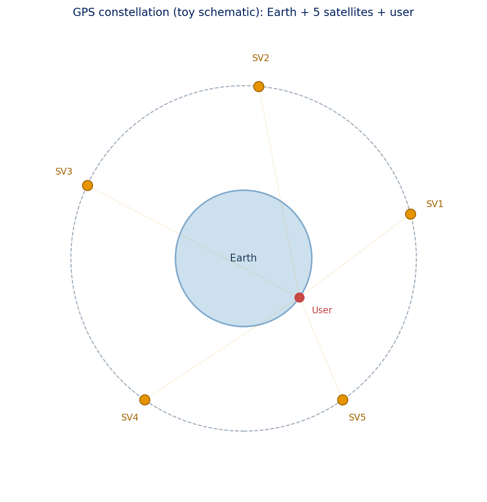
Fig. 1.1. Toy schematic of the GPS constellation. The signal from each satellite is faint by the time it reaches Earth (about \(-130\) dBm), which is why GPS is so easy to jam — that is one of the central topics of Block 8.

How GPS Measures Distance: The Pseudorange

A satellite transmits its PRN code at a precisely known time \(t_{\text{tx}}\). The receiver records when it hears the code arrive at \(t_{\text{rx}}\). The apparent travel time multiplied by the speed of light gives an apparent range:

\[ c \cdot (t_{\text{rx}} - t_{\text{tx}}). \]

There is one problem: the receiver’s clock is not synchronized to the satellite’s atomic clock. A receiver-clock offset \(\delta t_u\) (typically tens or hundreds of meters worth of time error) corrupts every measurement equally. The result is a pseudorange:

\[ \tilde{\rho}_i = \underbrace{\lVert \mathbf{r}_u - \mathbf{r}^{(i)} \rVert}_{\text{true range}} + c\, \delta t_u + \epsilon_i. \]

The “pseudo” in pseudorange refers to that clock-bias term. Each measurement is the true geometric range from user to satellite, plus the same unknown clock offset, plus measurement noise \(\epsilon_i\).

Key Concept

A pseudorange is a true range plus a common, unknown receiver-clock bias plus noise. The clock bias is just another unknown to estimate alongside position.

GPS as a Nonlinear Estimation Problem

A 3D receiver has four unknowns: \(\mathbf{x} = [x, y, z, \delta t_u]^{\top}\). Each satellite contributes one pseudorange equation:

\[ \tilde{\rho}_i = h_i(\mathbf{x}) + \epsilon_i, \qquad h_i(\mathbf{x}) = \lVert \mathbf{r}_u - \mathbf{r}^{(i)} \rVert + c\, \delta t_u. \]

The map \(h_i\) is nonlinear in user position because of the Euclidean norm. With four or more satellites visible, the system is over-determined and you can solve it as a nonlinear least-squares problem:

\[ \hat{\mathbf{x}} = \arg\min_{\mathbf{x}} \sum_i \left( \tilde{\rho}_i - h_i(\mathbf{x}) \right)^2. \]

There is no closed-form solution. Standard practice is iterative: Newton-Raphson, Levenberg-Marquardt, or any general-purpose nonlinear least-squares routine (MATLAB’s fitnlm, scipy’s least_squares). At each iteration you linearize \(h_i\) around the current best guess and take a step toward the minimum.

The GPS Positioning demo at the end of this block runs this exact procedure on a 2D toy GPS problem and lets you drag satellites around the orbit to watch the geometry effect happen live.

How Satellite Geometry Affects Accuracy

Each pseudorange defines a sphere of possible user positions, centered on the corresponding satellite. The user is at the intersection of those spheres. The shape of the intersection — sharp or smeared — depends entirely on the angles at which the spheres meet.

• Well-spread satellites in the sky produce spheres that cross at sharp angles. Their intersection is a tight cluster: small position uncertainty.

• Clustered satellites (all bunched in one part of the sky) produce spheres that are nearly parallel where they meet. The intersection smears out along the common line of sight: large position uncertainty.

Same pseudorange noise \(\sigma_\rho\), dramatically different position accuracy. The geometry does the amplifying.

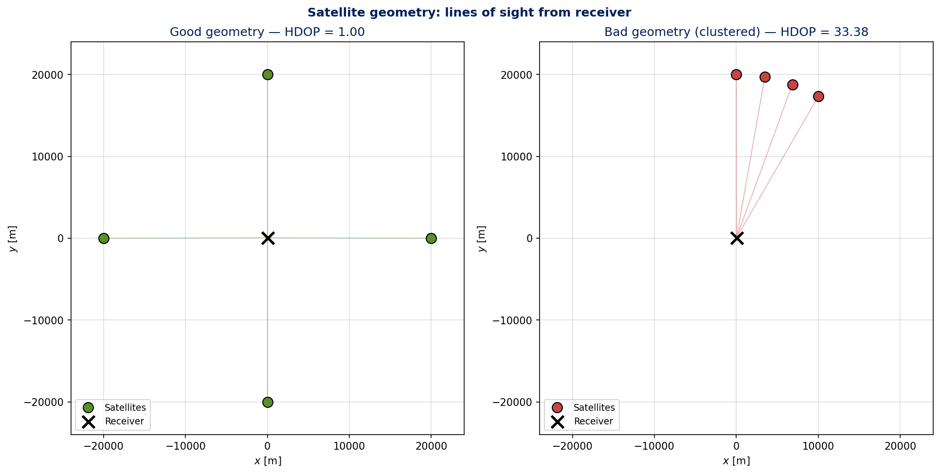
Fig. 1.2. Same number of satellites, same \(\sigma_\rho\), but the bad-geometry case has all four satellites within 30 degrees of each other. The bad case will produce a position estimate dramatically worse than the good case.

Dilution of Precision (DOP)

DOP quantifies the geometry effect with a single scalar. Define

\[ \sigma_{\text{position}} = \mathrm{DOP} \times \sigma_\rho. \]

Variants split the geometry contribution by component:

• HDOP (horizontal): horizontal position uncertainty per unit pseudorange noise.

• VDOP (vertical): vertical position uncertainty per unit pseudorange noise.

• PDOP (3D position): combined.

• TDOP (time): clock uncertainty.

Typical operating values:

• HDOP \(\approx 1\) to \(2\): good geometry, normal operation.

• HDOP \(> 4\): degraded accuracy, often flagged in receivers.

• HDOP \(\gg 4\): pathological geometry, position essentially unconstrained in some direction.

DOP is a property of geometry only. It does not depend on signal strength or receiver hardware. A precision receiver with \(\sigma_\rho = 0.5\) m and HDOP = 10 will report a position with \(\sigma_{\text{horiz}} = 5\) m. A consumer receiver with \(\sigma_\rho = 5\) m and HDOP = 1 will produce the same precision.

Key Concept

Geometry matters as much as pseudorange noise. \(\sigma_{\text{position}} = \mathrm{DOP} \times \sigma_\rho\) is the operational decomposition: receiver hardware controls \(\sigma_\rho\), the constellation controls DOP.

GPS Error Sources

Four physical effects dominate \(\sigma_\rho\) for a single-frequency civilian receiver.

Source	Typical magnitude	Mitigation
Ionospheric delay	1 to 5 m	Dual-frequency receivers; broadcast model corrections
Tropospheric delay	0.5 to 2 m	Saastamoinen model
Multipath	0.5 to 3 m	Antenna placement; signal-processing filters
Receiver noise	0.1 to 0.3 m	Hardware quality

Lumped together, \(\sigma_\rho \approx 3\) to 5 m for a typical L1 SPS (Standard Positioning Service) receiver. That number sets the diagonal entries of the measurement-noise covariance matrix \(\mathbf{R}\) when GPS gets folded into a Kalman filter (Block 7).

GPS Limitations

GPS is robust until it isn’t. The signal at Earth’s surface is roughly \(-130\) dBm — about a billionth the strength of a typical Wi-Fi signal. That weakness is the source of most operational problems:

• Jamming. A small-power transmitter on the right frequency overwhelms the satellite signal locally and denies positioning to every receiver in the area.

• Spoofing. Counterfeit signals that mimic real GPS broadcasts can mislead the receiver into reporting a wrong position. The threat is increasingly accessible; software-defined radios make spoofers buildable in a hobby lab.

• Denied environments. Indoors, underground, in urban canyons, under heavy foliage. The satellites are simply not visible.

• Vertical-versus-horizontal asymmetry. VDOP is usually worse than HDOP because GPS satellites only ever sit at or above the horizon. The receiver never sees a satellite “below” it, so the vertical component of the geometry is always partially under-constrained.

These limitations are the entire reason for the F-47 capstone problem in Block 10: when GPS goes down, the alternative-navigation stack must take over.

Quick Exercise

A GPS receiver tracks satellites with \(\sigma_\rho = 3\) m.

Scenario A: Satellites well spread, HDOP = 1.5. Scenario B: Satellites clustered, HDOP = 4.0.

Compute the horizontal \(1\sigma\) position accuracy for each scenario. Then a solar storm doubles \(\sigma_\rho\) to 6 m. What happens in each scenario?

Solution

Baseline (3 m). Scenario A: \(\sigma_{\text{horiz}} = 1.5 \times 3 = 4.5\) m. Scenario B: \(\sigma_{\text{horiz}} = 4.0 \times 3 = 12\) m.

Solar storm (6 m). Scenario A: \(\sigma_{\text{horiz}} = 1.5 \times 6 = 9\) m. Doubled, but still operationally usable. Scenario B: \(\sigma_{\text{horiz}} = 4.0 \times 6 = 24\) m. Bad-geometry case is now far outside operational tolerances.

The take-away: bad geometry doesn’t just give you a worse baseline; it amplifies any increase in pseudorange noise more aggressively than good geometry. That is why operational receivers display a DOP figure alongside the position fix, and why navigation filters typically gate measurements through a DOP threshold before accepting them.

GPS Positioning Demo

The GPS Positioning demo in this block solves the 2D nonlinear-least-squares fit on a draggable satellite constellation. A constellation overview lets you reposition each satellite around the orbit; a synchronized receiver-area zoom shows the pseudorange bands (each one a tangent line to the satellite’s range circle, drawn perpendicular to the line of sight) and the resulting 95% covariance ellipse. Geometry presets (Even spread, Clustered, Half sky, Pole + cluster) let you flip between dramatically different HDOP regimes in one click — the same number of satellites and the same per-pseudorange noise can produce position accuracy that differs by 10–30× depending purely on how the satellites are arranged in the sky. A MATLAB implementation is also included at code/GPSPositioningDemo.m.

Wrap-Up

GPS measures pseudoranges, not positions. Each pseudorange is a true geometric range plus a common, unknown receiver-clock bias plus noise. With four or more satellites visible, the receiver solves a nonlinear least-squares problem to recover position and clock bias simultaneously. Satellite geometry amplifies pseudorange noise into position error through DOP: \(\sigma_{\text{position}} = \mathrm{DOP} \times \sigma_\rho\). Pseudorange noise itself is dominated by ionospheric, tropospheric, multipath, and receiver-noise contributions, lumping to a few meters for an L1 SPS receiver. Operational limits — jamming, spoofing, denied environments, and weak vertical geometry — make GPS a critical but never-sufficient navigation source.

The next block tackles the obvious downstream question: GPS measurements are nonlinear in user position, so they cannot feed directly into the linear Kalman filter of Block 5. The Extended Kalman Filter linearizes \(h_i\) once per cycle around the current best estimate, and that is what gets the pseudorange machinery into the filter framework.