Block 2 — Inertial Error Growth and State Propagation

By the end of this block you should be able to:

1. Explain why inertial navigation errors grow over time.

2. Trace how small sensor errors propagate into velocity and position errors.

3. Identify the common error models used in navigation systems: bias, random walk, and Gauss-Markov.

4. Define the navigation state and explain what state propagation does.

5. Interpret inertial drift using simple operational metrics, including drift slope in NM/hr and the role of the Schuler cycle.

What an IMU Measures

An Inertial Measurement Unit (IMU) is a tightly coupled assembly of accelerometers and gyroscopes that gives a navigation algorithm two raw, high-rate signals:

• Specific force from the accelerometers, which is gravity-compensated linear acceleration along each body axis.

• Angular rate from the gyroscopes, which is the body’s rotation rate about each body axis.

Both measurements are expressed in the body frame. To produce position, velocity, and attitude in NED, the navigation algorithm has to integrate angular rate to track attitude, rotate the gravity-compensated accelerations into NED, and then integrate twice to get velocity and position. This procedure is called mechanization, and it is where small sensor errors become big navigation errors.

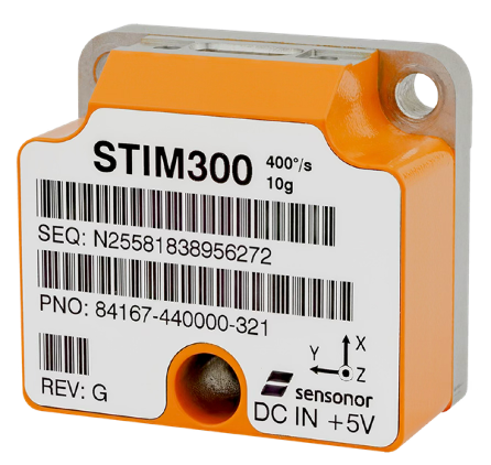
Fig. 2.1. The STIM300 is the tactical-grade IMU used in the F-47 alternative-nav stack you will analyze in Block 10. The course reference materials include its datasheet.

The Inertial Error Integration Chain

Every IMU error rides through the same pipeline:

Sensor error	First integration	Second integration
Accelerometer error	Velocity error	Position error
Gyroscope error	Attitude error → wrong gravity projection → secondary acceleration error	… which then integrates again

The accelerometer chain is direct: an offset on the measured specific force becomes velocity error after one integration and position error after two. The gyroscope chain is indirect but more dangerous: an attitude error tips the gravity vector into the horizontal plane, which produces a non-zero horizontal acceleration error that then integrates into velocity and position. This indirect path is what gives inertial errors their characteristic Schuler oscillation later in this block.

Key Concept

Inertial drift is the result of integrating imperfect measurements. Every sensor error becomes a navigation error of higher order in time.

Common Inertial Error Types

Three error types show up in nearly every IMU specification.

Bias is a constant offset on a measurement. A constant accelerometer bias of \(0.02 \text{ m/s}^2\) produces a velocity error that grows linearly with time and a position error that grows quadratically.

Random noise is sample-to-sample variation around the true value. White-noise velocity error integrates into a random-walk position error whose RMS grows like \(\sqrt{t}\).

Drift is the catch-all term for accumulated navigation error over time. It includes both deterministic (bias-driven) and stochastic (noise-driven) contributions.

The Inertial Error Integration demo in this block lets you inject any of the four canonical error processes (constant bias, white noise, random walk, Gauss-Markov) at either the acceleration or velocity level, and watch the result integrate forward into velocity and position errors. A MATLAB implementation is also included at code/ErrorIntegrationDemo.m.

Simple Error Models

To predict navigation performance without modeling every physical detail, we use compact statistical models for sensor errors.

Random walk

A first-order random walk on a sensor bias is a discrete-time model where the bias takes a small random step every sample:

\[ b_{v,k+1} = b_{v,k} + w_k, \qquad w_k \sim \mathcal{N}(0, q\, \Delta t). \]

The bias has no preferred value and its variance grows linearly with time. Random walk is the right model for many gyro-related errors that have no natural decay mechanism.

Gauss-Markov (correlated noise)

A first-order Gauss-Markov process adds a decay term, so the error has a finite “memory” set by a correlation time \(T\):

\[ x_{k+1} = e^{-\Delta t / T}\, x_k + w_k. \]

For \(\Delta t \ll T\) the error behaves like a slow random walk. For \(\Delta t \gg T\) it behaves like white noise. Most accelerometer biases and many environmental errors are well-fit by Gauss-Markov, which is why it is the workhorse model for navigation covariance budgets.

Key Concept

Error models capture the statistics of sensor behavior without modeling every physical detail. They are the bridge between a datasheet specification and a covariance you can actually propagate.

We will revisit Gauss-Markov in Block 5 when we build a 6-state filter that tracks acceleration as a Gauss-Markov state.

Allan Variance: Characterizing IMU Errors on the Ground

The error models above (random walk, Gauss-Markov) need real numbers to be useful. The standard tool for getting those numbers is Allan variance, and it is a ground test, not a flight test: a long static IMU run, typically about 6 hours, measured before any aircraft ever leaves the ramp.

The reason this works is that a static IMU should report zero specific force in the horizontal channel and zero angular rate. Anything else is sensor error. By looking at how the variance of the measured signal evolves as you average it over different cluster times \(\tau\), you can separate the underlying error processes:

• White noise — angle random walk (ARW) on gyroscopes, velocity random walk (VRW) on accelerometers.

• Bias instability — the slow, low-frequency wander in the bias that no calibration ever fully removes.

• Rate random walk / acceleration random walk — the long-term drift of the bias itself.

• Quantization noise — discrete-output artifacts at the shortest cluster times.

Each of these processes shows up as a different slope on a log-log plot of Allan deviation \(\sigma(\tau)\) versus cluster time \(\tau\):

• Slope \(-1/2\): white noise (ARW or VRW).

• Slope \(0\): bias instability — the floor of the Allan curve.

• Slope \(+1/2\): rate random walk.

So an Allan deviation plot reads like a fingerprint: identify the slope segments and you have separated the noise sources contributing to the IMU output.

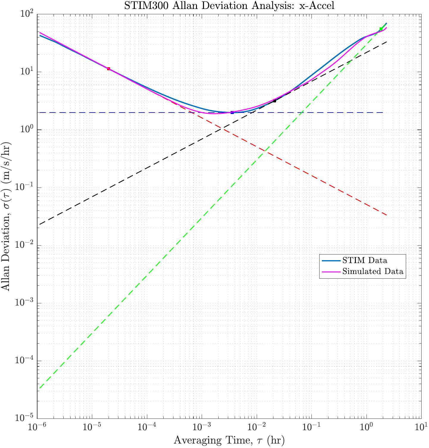
Fig. 1.1. Allan deviation analysis of the STIM300 x-axis accelerometer. The blue curve is real STIM300 data; the magenta is a simulated model fit to it. The dashed lines mark the canonical \(-1/2\), \(0\), and \(+1/2\) slopes that identify each underlying noise process. The minimum of the curve sets the bias-instability floor.

Key Concept

Allan variance is a ground test, not a flight test. A long static run (typically about 6 hours) is enough to fingerprint the IMU’s error processes by their distinct slopes on the Allan deviation plot. The numbers it produces flow straight into the Kalman filter’s \(\mathbf{Q}\) and bias-state models.

Why we care for the rest of the course

Allan variance numbers are the bridge from a vendor datasheet to a working navigation filter:

1. The white-noise slope gives ARW / VRW values that go directly into the \(\mathbf{Q}\) matrix on the position and velocity states.

2. The bias-instability floor and the rate-random-walk slope decide whether you model an axis bias as a random walk (longer correlation time) or a Gauss-Markov process (finite correlation time), and what time constant to use.

3. The full Allan curve determines how quickly the INS will drift in the absence of aiding, which sets your floor expectation on the F-47 ANS inertial-only requirement (Block 9 / Project, \(\le 1.0\) NM/hr at the upper 95% CI).

You will see the STIM300 datasheet numbers (Allan variance derived) referenced again in Block 9 when we plan the developmental-test campaign, and in the project when we benchmark the F-47 ANS against its requirements. The Additional References section in the sidebar contains the full Allan variance reference article and the STIM300 datasheet for deeper reading.

The Navigation State

Navigation algorithms estimate a state vector. A typical 9-state form is

\[\begin{split} \mathbf{x} = \begin{bmatrix} \mathbf{p} \\ \mathbf{v} \\ \mathbf{a} \end{bmatrix}, \end{split}\]

with position \(\mathbf{p} \in \mathbb{R}^3\), velocity \(\mathbf{v} \in \mathbb{R}^3\), and an attitude representation \(\mathbf{a} \in \mathbb{R}^3\) (commonly small-angle tilt error or roll-pitch-yaw). The estimator pairs this with a state error covariance

\[ \mathbf{P} \in \mathbb{R}^{9 \times 9} \]

that quantifies how trustworthy each component is and, crucially, how the components are correlated. A position error correlated with an attitude error tells you a lot about whether a measurement update will fix one when it corrects the other; we will see that explicitly when we build the multi-state Kalman filter in Block 5.

State Propagation

Navigation algorithms repeatedly propagate the state forward in time using a motion model and the latest IMU measurements:

\[ \mathbf{x}_{k+1} = f(\mathbf{x}_k, \mathbf{u}_k) + \mathbf{w}_k, \]

where \(\mathbf{u}_k\) is the IMU measurement vector and \(\mathbf{w}_k\) is process noise that captures everything the motion model does not. The covariance propagates with it, using the Jacobian \(\mathbf{F}_k = \partial f/\partial \mathbf{x}\) and a process-noise covariance \(\mathbf{Q}_k\):

\[ \mathbf{P}_{k+1} = \mathbf{F}_k\, \mathbf{P}_k\, \mathbf{F}_k^{\top} + \mathbf{Q}_k. \]

This is the propagation half of every Kalman filter. The take-away is that uncertainty grows over time when the only information feeding the algorithm is a noisy IMU. The other half of the Kalman filter, the measurement update, is what reins it back in. We will derive it in Block 4.

Quick Exercise

Suppose a constant accelerometer bias of \(b_a = 0.02 \text{ m/s}^2\) produces a constant acceleration error in your navigation solution.

1. What does the velocity error look like as a function of time?

2. Does the position error grow linearly or quadratically?

3. After 60 seconds of free inertial coast, what is the position error?

4. What changes if the system receives a position fix every 30 seconds?

Solution

(1) \(v_e(t) = b_a t\), linear growth at \(0.02 \text{ m/s}^2 \times t\). After 60 s, \(v_e = 1.2 \text{ m/s}\).

(2) Position error is the integral of velocity error: \(p_e(t) = \tfrac{1}{2} b_a t^2\), quadratic.

(3) \(p_e(60) = \tfrac{1}{2} \cdot 0.02 \cdot 60^2 = 36 \text{ m}\).

(4) Each fix bounds the position error by the fix accuracy (and indirectly bounds velocity error too, through the filter’s cross-covariance). Between fixes, the same quadratic growth resumes from the post-fix state. The time-averaged position error is dramatically smaller because the quadratic growth is reset before it can run away. This is the entire motivation for fusing inertial with an aiding sensor.

Why Inertial Drift Tests Are Long

Horizontal inertial errors do not just grow monotonically. They oscillate at the Schuler period, named after Maximilian Schuler, who showed that an inertial system tuned to the radius of the Earth has a natural oscillation period

\[ T_{\text{Schuler}} = 2\pi \sqrt{\frac{R_e}{g}} \approx 84.4 \text{ min}. \]

To characterize inertial drift you need to observe at least one full Schuler cycle, otherwise your slope fit will be biased by whatever phase of the oscillation you happen to be on when you stop the test. The practical rule of thumb in flight test:

Key Concept

Inertial drift runs should be at least 85 minutes long. Anything shorter and your drift estimate is corrupted by where the Schuler oscillation happens to be.

Why the Schuler Cycle Happens

The mechanism is straightforward once you trace through the integration chain.

1. Suppose the nav solution has a small attitude error \(\theta\).

2. Gravity, which the algorithm thinks points along body \(-Z\), now has a horizontal projection of approximately \(g\theta\).

3. The mechanization removes a slightly wrong gravity vector and reports a non-zero horizontal acceleration that does not exist.

4. That false acceleration integrates into a velocity error, which integrates into a position error, which (via the way the algorithm levels itself against gravity) feeds back to correct the attitude error.

5. The system overshoots and corrects, and you have an oscillator.

The natural frequency of that oscillator is set by Earth’s gravity and radius, which is what gives you the universal 84.4-minute period.

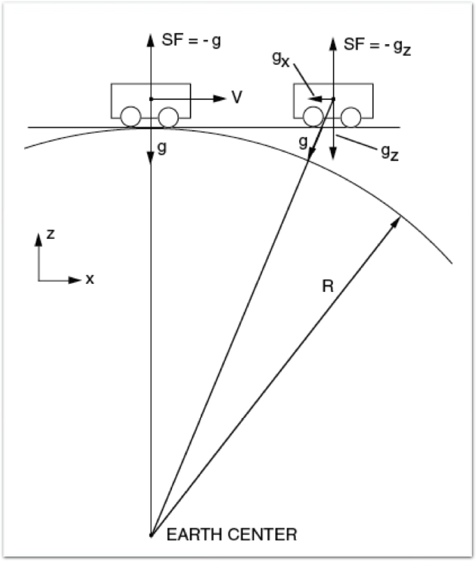
Fig. 2.2. The Schuler oscillation arises from the closed loop between attitude error, mis-projected gravity, horizontal velocity error, and the algorithm’s level-correction logic. The course reference materials include a more rigorous derivation.

Inertial Drift Demo

The interactive Inertial Drift demo in this block simulates a long-run horizontal error signal of the form

\[ e_H(t) = b\, t + A \cos(\omega t + \phi_0) + v(t), \]

with \(b\) a true drift slope, \(A \cos(\omega t + \phi_0)\) a Schuler oscillation, and \(v(t)\) measurement noise. The demo plots the entire time history with the slope fit using only the first \(W\) minutes, alongside a drift-vs-window curve that shows what the OLS slope estimate would be for every possible window length on the same data. The curve oscillates around truth with period \(T_S/2\) and converges to truth at integer multiples of \(T_S\) — the operational reason inertial drift tests are sized in Schuler cycles, not minutes. A MATLAB implementation is also included at code/InertialDriftDemo.m.

Wrap-Up

Inertial navigation integrates IMU measurements to estimate motion, and small sensor errors accumulate through that integration. Bias, random walk, and Gauss-Markov are the three workhorse error models that connect a datasheet to a covariance. The state propagates forward via a motion model, and its covariance grows alongside it through the \(\mathbf{F}\mathbf{P}\mathbf{F}^{\top} + \mathbf{Q}\) recursion. Drift in the unaided horizontal channel is dominated by an 84.4-minute Schuler oscillation, which sets a hard lower bound on how long an inertial-only test must run.

The next block looks at the obvious counter-question: if inertial drift is unavoidable on its own, can a second sensor bound it? That is optimal fusion, and it is the bridge to the Kalman filter.