Block 8 — Fault Detection, Integrity, and HMI#
By the end of this block you should be able to:
Define a sensor fault and explain why it causes the Kalman filter innovation to grow.
Apply the Mahalanobis distance test to determine when an innovation is statistically suspicious.
Distinguish between filter error bounds (from \(\mathbf{P}\)) and integrity bounds (protection levels).
Define Hazardous Misleading Information (HMI) and identify it from position-error and protection-level time histories.
What Is a Sensor Fault?#
A fault is any condition where a measurement no longer behaves according to the assumed model:
When the assumption fails, the filter has no way to know the measurement is no longer trustworthy. It folds the corrupted measurement into the state estimate just like any other, and the resulting state slowly drifts away from truth. Common fault sources in GPS and inertial navigation:
Spoofing or jamming. An adversary injects a deliberate range bias into one or more pseudoranges.
Unmodeled bias. Satellite-clock anomalies, thermal drift, multipath.
Wrong model parameters. Incorrect lever-arm calibration, timing offset, scale factor.
Geometry collapse. Satellite dropout, sudden PDOP spike that the filter’s \(\mathbf{R}\) does not capture.
Key Concept
A fault is not “extra noise”. A fault violates the distributional assumptions of the estimator. The filter ingests it silently and corrupts its state estimate without raising any internal flag.
The Innovation Under a Fault#
Under healthy conditions the innovation \(\boldsymbol{\nu}_k = \mathbf{z}_k - h(\hat{\mathbf{x}}_k^-)\) is zero-mean Gaussian with covariance \(\mathbf{S}_k\). Under a slowly-growing ramp fault \(b_f(t_k)\) on one pseudorange, the measurement becomes \(z_k = h(\mathbf{x}_k) + v_k + b_f(t_k)\) and the innovation picks up a steadily growing bias:
The crucial point is that the innovation variance \(S_k = \mathbf{H}\mathbf{P}^-\mathbf{H}^{\top} + \sigma_\rho^2\) does not change. It is computed from the filter’s internal model of itself, and the model has no idea anything is wrong. So the innovation grows steadily while \(S_k\) stays small — and the ratio \(\nu_k / \sqrt{S_k}\), which is the “sigma count” the filter considers normal, blows up.
That ratio is exactly what fault detection tests against.
How Big Is Too Big? Mahalanobis Distance#
In one dimension, deciding whether a residual is suspicious is straightforward: count sigmas. \(|\nu|/\sigma > 3\) is a 3-sigma event, expected to happen with probability about \(0.27\%\) under the null hypothesis. With vector-valued measurements we need a generalization that accounts for the full innovation covariance \(\mathbf{S}\), not just its diagonal entries.
Mahalanobis distance is the natural generalization:
This single scalar weights each component of the innovation by its uncertainty, accounts for correlations between components, and reduces to \((\nu/\sigma)^2\) in the scalar case. It is dimensionless: a \(D^2\) value of 4 means “the innovation sits at the 2-sigma boundary of the joint Gaussian”, regardless of how many components \(\boldsymbol{\nu}\) has.
Key Concept
Mahalanobis distance is the “how many sigmas” question for vector innovations. It accounts for both the variance scale and the correlation structure of \(\mathbf{S}\).
Detection as a Hypothesis Test#
Under healthy conditions, the Mahalanobis distance follows a chi-squared distribution:
where \(m\) is the number of measurement components stacked into \(\boldsymbol{\nu}\). The decision rule is
The threshold \(\gamma\) is set by the desired false-alarm probability \(P_{\text{FA}}\):
Number of measurements \(m\) |
\(P_{\text{FA}} = 1\%\) |
\(P_{\text{FA}} = 0.3\%\) |
|---|---|---|
1 (single pseudorange) |
6.63 |
8.83 |
4 (batch, 4 satellites) |
13.28 |
16.25 |
30 (running 30-sec window at 1 Hz) |
43.77 |
49.95 |
A tighter threshold (smaller \(\gamma\)) catches faults faster but raises the false-alarm rate. A looser threshold reduces false alarms but increases time-to-detect on slow faults. The whole game in fault detection is choosing where to sit on this curve.
Quick Exercise: Is This Residual Suspicious?
Satellite 1 has a ramp fault with rate \(\dot{b}_f = 3\) m/s injected at \(t_0 = 10\) s. The innovation variance is \(S = 25\) m\(^2\) (so \(\sigma_S = 5\) m).
(a) At \(t = 15\) s the pseudorange innovation is \(\nu = 15\) m. Compute \(D^2 = \nu^2 / S\). Is this suspicious at \(P_{\text{FA}} = 0.3\%\) (\(m = 1\), \(\gamma = 8.83\))?
(b) The bias grows linearly from zero. At what time does \(D^2\) first exceed \(\gamma = 8.83\)? What is the time-to-detect \(T_D = t_D - t_0\)?
(c) If you tighten the threshold to \(\gamma = 4.0\), what happens to \(T_D\)? What is the cost?
Solution
(a) \(D^2 = 15^2 / 25 = 9\). This sits just above \(\gamma = 8.83\), so yes, it is statistically suspicious at the \(P_{\text{FA}} = 0.3\%\) level.
(b) The bias at time \(t\) is \(b_f = 3(t - 10)\). The innovation tracks this bias plus zero-mean noise, so we ask when the mean innovation crosses the detection bound: \(\sqrt{\gamma\,S} = \sqrt{8.83 \cdot 25} \approx 14.85\) m. Setting \(3(t - 10) = 14.85\) gives \(t_D \approx 14.95\) s, so \(T_D \approx 5\) s. (In practice the noise term means \(D^2\) might cross slightly earlier or later, but 5 s is the deterministic mean.)
(c) With \(\gamma = 4.0\), the detection threshold drops to \(\sqrt{4 \cdot 25} = 10\) m, so \(t_D = 10 + 10/3 \approx 13.3\) s and \(T_D \approx 3.3\) s. About 1.7 s faster. The cost: \(P_{\text{FA}}\) at \(\gamma = 4\) for a 1-DOF chi-squared is about \(4.6\%\) — fifteen times higher than the original \(0.3\%\). Faster detection, more false alarms.
What Happens After Detection?#
Detection alone does not solve the problem; the system has to respond. Common patterns:
Fault exclusion. Drop the offending satellite and continue with the remaining ones. Works if you have at least four others visible.
Fault accommodation. Inflate the offending sensor’s \(\mathbf{R}\) entry so the filter de-weights it, or augment the state with an explicit bias for that sensor that the filter can estimate out.
Fault recovery. Re-introduce the sensor once its innovations return to nominal levels for some confirmation period.
Multi-filter / parallel hypothesis. Run \(N\) sub-filters in parallel, each excluding one satellite. The sub-filter that stays statistically consistent identifies the culprit, because excluding the bad satellite removes the source of the bias.
The F-47 ANS in the Block 10 capstone uses a multi-filter architecture: one main filter plus sub-filters each excluding one sensor. The output that drives the integrity decision is separate from the main filter’s covariance \(\mathbf{P}\).
Filter Error Bounds vs. Integrity Bounds#
The filter covariance \(\mathbf{P}\) produces an error ellipse: “if the model is correct, the true error lies inside this ellipse with high probability.” The trouble is that an undetected fault corrupts \(\hat{\mathbf{x}}\) but does not grow \(\mathbf{P}\). The filter has no idea anything is wrong, so its \(\mathbf{P}\) stays small and the ellipse becomes inconsistent — the actual error no longer lives inside it.
The integrity bound is a separate, more conservative bound, computed from the multi-filter architecture rather than from the main filter’s covariance. It is designed to remain valid even when one sensor is faulty, because the sub-filter that excludes the faulted sensor still has good information.
In a healthy system, the truth sits inside both the filter’s \(\mathbf{P}\) ellipse and the integrity bound. In a faulty-but-undetected system, the truth has drifted outside the filter’s \(\mathbf{P}\) ellipse (the filter is “confidently wrong”) but is still inside the integrity bound — that is the safe outcome.
Protection Levels#
The integrity bound is reported as usable spatial thresholds called protection levels.
Horizontal Protection Level:
Vertical Protection Level:
Here \(P_{\text{int}}\) is the diagonal of the integrity covariance (from the multi-filter architecture, not the main filter’s \(\mathbf{P}\)), and \(n_\alpha\) is the multiplier for the desired containment probability — for example \(n_\alpha = 2.576\) for a 99% bound.
HPL and VPL are not confidence ellipses from the EKF. They are guaranteed performance zones from the multi-filter architecture, valid under a single-sensor fault. That distinction is what makes them suitable for safety-of-life applications like aviation precision approach.
Hazardous Misleading Information (HMI)#
HMI is the most important failure mode in any safety-critical navigation system. It is defined as the condition where the true position error exceeds the protection level while the fault is still undetected:
In words: the system is actively misleading the operator. It is reporting a position with a tight protection-level guarantee, the operator believes that guarantee, but truth is actually outside the bound. This is the scenario any integrity-monitoring system must prevent or at least detect quickly.
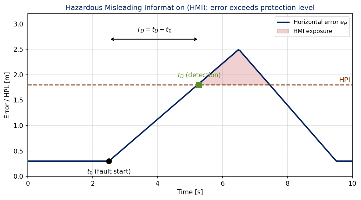
Fig. 3.1. The two operational quantities every integrity test report tracks: (1) time-to-detect \(T_D = t_D - t_0\), the elapsed time between the fault starting and the system declaring it detected; (2) HMI exposure, the total time during which the true error exceeds the protection level. The F-47 ANS Requirement 4 in Block 10 sets a \(T_D \le 5\) s threshold and an HMI-exposure \(\le 1\) s threshold, with both being bounded events the test must observe.
Spoof Detection in Action#
The two short videos below come from our research-lab visualization of a tightly-coupled GPS/INS filter under spoof attacks. They show the time-history of position error, protection level, and the per-satellite Mahalanobis distance as the spoof injection grows. Watch for the moment the per-satellite \(D^2\) trace climbs above the threshold and the protection level inflates to keep the truth inside.
Single-satellite spoof event. One pseudorange picks up a slowly-growing bias. The per-satellite \(D^2\) for that one channel diverges from the chi-squared distribution while the others stay nominal. Sub-filter isolation flags the offender within a few seconds and the integrity solution holds the protection level wider while the bad satellite is downweighted.
Two-satellite spoof event. With more than one satellite faulted simultaneously, simple per-satellite testing is no longer enough — multiple \(D^2\) traces light up. The multi-filter architecture has to consider sub-filters that exclude multiple satellites, and the integrity bound widens accordingly. This is the scenario the F-47 ANS multi-filter design is meant to handle.
Fault Detection Demo#
The Fault Detection demo in this block extends the 5-state EKF from Block 7 with GPS fault injection and three coupled chi-squared monitoring views: the per-sample \(D^2_k\) test, the running \(M\)-sample \(\sum D^2_k\) test, and a full sub-filter isolation matrix. A live trajectory shows the main filter drifting away from truth while the sub-filter that excluded the faulted satellite stays clean. Sliders let you change the faulted SV, the ramp rate \(\dot{b}_f\), and the window length \(M\) to explore the false-alarm-vs-time-to-detect trade. The pedagogy is deliberately ungilded — neither the trajectory legend nor the isolation matrix tells you which sub-filter is the clean one; you read the chi-squared structure yourself. A MATLAB implementation is also included at code/FaultDetectionDemo.m.
Wrap-Up#
A sensor fault violates the measurement model and the filter ingests it silently; the state estimate corrupts while the covariance stays misleadingly tight. The innovation grows under a fault while \(\mathbf{S}\) does not, so the Mahalanobis distance \(D^2 = \boldsymbol{\nu}^{\top}\mathbf{S}^{-1}\boldsymbol{\nu}\) is a clean test statistic with a known chi-squared distribution under the null. Detection is a hypothesis test against a chi-squared threshold, with \(P_{\text{FA}}\) trading against time-to-detect. Integrity is a separate question from accuracy: protection levels (HPL, VPL) come from a multi-filter architecture and remain valid under single-sensor faults, while the main filter’s \(\mathbf{P}\) becomes inconsistent. HMI — true error exceeding the protection level — is the failure mode any integrity-monitoring system must prevent or quickly detect. The F-47 ANS capstone in Block 10 will require you to measure \(T_D\) and HMI exposure on a 30-event spoof dataset, against a \(T_D \le 5\) s threshold and an HMI-exposure \(\le 1\) s threshold.
Block 9 introduces the project framing: how to plan a statistically defensible flight-test campaign for a navigation system, including correlation time, effective sample size, and the autocorrelation discount you have to apply when working with high-rate sensor data.