Block 4 — Scalar Kalman Filter#
By the end of this block you should be able to:
Explain how the Kalman filter performs recursive optimal fusion.
Identify the roles of prediction, measurement, and innovation.
Interpret the Kalman gain as an uncertainty-weighted trust factor.
Update both the state and its uncertainty at every step.
Run the full predict-update cycle on a one-dimensional example.
The Recursive Estimation Problem#
In Block 3 we fused two simultaneous measurements of the same quantity. Real navigation systems do not get all their information at once. They run continuously, accumulating information over time. At every time step \(k\) the filter has two pieces of input:
A prediction of the state and its uncertainty, propagated forward from the previous step:
A new measurement with its own uncertainty:
The goal is to fuse these two optimally, producing an updated state \(\hat{x}_k^+\) and a posterior covariance \(P_k^+\). Then propagate forward again, and repeat. That recursion is the Kalman filter.
Key Concept
A Kalman filter is two things stitched together: optimal fusion of a prior and a measurement, and a rule for moving the prior forward in time. Both halves carry the state and its covariance; you cannot do one without the other.
The Innovation#
Define the innovation as the difference between the measurement and what the prior predicted you would see:
The innovation is the new information the measurement carries. A small innovation says the prediction was already close to the measurement, so there is little to learn. A large innovation says the measurement is telling you something the prediction missed.
The innovation has its own variance, made up of the prediction uncertainty \(P_k^-\) and the measurement uncertainty \(R_k\):
We will use \(S_k\) later when we build the chi-squared fault detection test in Block 8.
The Kalman Gain#
The Kalman gain is the optimal weight on the innovation when updating the estimate. For the scalar case it is
Notice that this is exactly the inverse-variance weight from Block 3, with the prior playing the role of “sensor 1” and the measurement playing the role of “sensor 2”. The Kalman gain is just optimal fusion in disguise.
The interpretation of the gain is straightforward:
\(P_k^- \gg R_k\) (prediction uncertain, measurement trustworthy): \(K_k \to 1\). The filter pulls the estimate hard onto the measurement.
\(R_k \gg P_k^-\) (prediction trustworthy, measurement noisy): \(K_k \to 0\). The filter mostly ignores the measurement.
Everywhere in between, \(K_k\) blends the two with the optimal trust factor.
Key Concept
The Kalman gain is a trust factor between zero and one. When you see a confusing filter behavior, look at the gain time history first. It tells you what the filter believed at every step.
State and Covariance Update#
With the gain in hand, the state update is
The covariance update for the scalar filter is
Because \(0 \le K_k \le 1\), the posterior covariance is always smaller than the prior. The measurement update never increases uncertainty — that is the whole point of incorporating new information.
The general matrix form (Joseph form, used to keep \(P^+\) symmetric and positive-definite under finite-precision arithmetic) is
which we will revisit in Block 5 when the state becomes a vector.
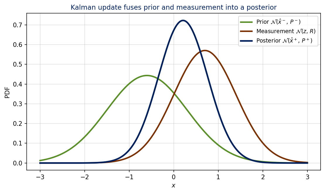
Fig. 1.1. The Kalman update is the Gaussian-on-Gaussian product. The posterior mean sits between the two inputs, weighted by their respective inverse variances; the posterior variance is smaller than either input.
The Prediction Step#
Between measurements the filter has to march the state forward in time using a motion model. For a scalar state with linear dynamics:
\(F\) is the state transition factor. \(Q_k\) is the process-noise variance that captures everything the deterministic propagation model fails to represent: unmodeled disturbances, model mismatch, sensor noise that gets folded into the propagation. Set \(Q\) too small and the filter will be over-confident and ignore real measurements; set \(Q\) too large and it will follow noise instead of structure. Tuning \(Q\) against truth data is part of every real navigation deployment.
In the limit \(Q = 0\) and the prediction is exact, \(P^-\) stays the same as \(P^+\) from the last step. With a non-zero \(Q\) the predicted covariance grows monotonically until the next measurement arrives.
Key Concept
Prediction grows uncertainty. Measurement update shrinks it. The whole filter is a tug-of-war between \(Q\) and \(R\), and the steady-state Kalman gain settles wherever those two forces balance.
The Scalar Kalman Filter Cycle#
Pulling the four equations together gives the canonical predict-then-update cycle that runs once per time step:
Prediction \((k \rightarrow k+1)\):
Update \((- \rightarrow +)\):
If a step has no measurement (sensor offline, occluded, between samples), skip the update and leave \(\hat{x}^+, P^+\) equal to \(\hat{x}^-, P^-\). The prediction step still runs, and the covariance grows.
Quick Exercise
Given:
Compute the Kalman gain \(K\), the updated estimate \(\hat{x}^+\), and the posterior variance \(P^+\).
Solution
Kalman gain:
Updated estimate:
Posterior variance:
The measurement was more trustworthy than the prediction (\(R < P^-\)), so the gain is large and the estimate moves substantially toward the measurement. The posterior \(\sigma\) of about 2.57 m is smaller than either the prior \(\sigma\) of 5 m or the measurement \(\sigma\) of 3 m, which is the inverse-variance fusion result from Block 3.
Scalar Kalman Filter Demo#
The Scalar Kalman Filter demo in this block runs the canonical 1D Kalman filter on a moving-train scenario: noisy position measurements every 10 s, constant-velocity propagation between measurements, deliberately bad initial estimate so you can watch the filter find truth. A live track view at the top animates the train, the estimate, and the current ±95% covariance bar; three time-series panels (position, error, Kalman gain) show the full history with a synchronized “now” cursor.
Sliders let you change the measurement noise, the process noise, the update interval, and the initial conditions while the animation runs, so you can see directly:
the gain converging to a steady-state value as the filter learns how much to trust each new measurement;
the bounds widening between updates and snapping tighter at each update, the visible signature of \(P^- = P^+ + Q\,\Delta t\) alternating with \(P^+ = (1-K)P^-\);
the structural bias that appears when the model velocity differs from truth — a tight confidence interval does not protect you from a wrong model.
A MATLAB implementation is also included at code/KalmanFilterScalar.m.
Wrap-Up#
The Kalman filter is recursive optimal fusion. It carries a state and a covariance, propagates them forward via a motion model that grows uncertainty by \(Q\), and fuses each new measurement with a gain that is just the inverse-variance weight from Block 3. Innovation is the new information; the gain is how much you trust it; the posterior covariance is always smaller than the prior. That five-equation cycle is the foundation of every navigation filter you will build in the rest of the course.
The next block extends to vector states: position, velocity, attitude, with cross-covariance terms that propagate information between channels even when only one channel is being measured.