🔬 Lab 16 Tachometer#
📌 Objectives#
Students should be able to configure Timer_A module for input capture measurements.
Students should be able to develop low-level software drivers to measure distance and speed of the two motors on the robot.
Note
Simplicity is the soul of efficiency. – Austin Freeman
📜 Synopsis#
In this lab, we will develop a software module that measures the speeds of motors and the displacement of the robot. The key element for measuring the speed and displacement of our robot is a Hall-effect sensor, a semiconductor device that produces a voltage proportional to the magnetic field. As shown in the figure below, a Hall-effect sensor can measure the magnetic field intensity of two magnets attached to a rotating plate.
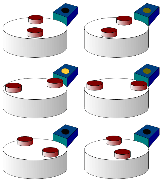
Our first objective in this lab is to develop Timer_A software capable of measuring periods from two encoders. The counter of Timer_A is 16 bits wide, which means our period measurements will have a precision of 16 bits, allowing us to measure 65,536 different periods.
The term resolution here refers to the smallest period that our measurement system can distinguish. When operating in input capture mode, this resolution is determined by the period of the selected clock. For example, if we choose the SMCLK clock running at 12 MHz, with a prescale of 1 and an input divider of 1/8, the period measurement resolution will be 2/3 microseconds. This means that the system can detect periods as small as 2/3 microseconds. With this configuration, the maximum measurable period is determined by the product of precision and resolution, which equals roughly 43 milliseconds (65,536 \(\times\) 2/3 \(\mu s \approx\) 43 ms).
The second objective of this lab is to utilize the measured periods to determine the wheel speed. Given that there are 360 pulses per rotation, the 43 ms maximum measurement period corresponds to the slowest wheel speed we can accurately measure, which is about 3.81 revolutions per minute (rpm).
We can calculate the angular speed of the wheel, denoted as \(\omega\) in rpm, using the following formula:
where \(n\) is the period in units of 2/3 microseconds. This formula allows us to convert the measured periods into angular speed in rpm.
The third objective involves utilizing the second input of the encoder to determine the direction of the motor’s rotation. This entails developing software that keeps track of the number of pulses detected on each wheel as the robot advances. As the robot moves forward, these pulses will be added to a counter, and as it moves backward, pulses will be subtracted from the counter. Subsequently, this counter will play a crucial role in determining the distance traveled.
💻 Procedure#
Setup#
If you haven’t already, download
TimerA2.cfrom Teams > General > Files > Class Materials > SourceFiles. Move it to theincfolder to replace the existing file with the same name.Download
Lab16_Tachmain.cfrom the same location. Move it to theLab16_Tachfolder to replace the existing file.Download
TA3InputCapture.[c,h]andTachometer.[c,h]from the same location. Move them to theincfolder to replace the existing file.
Complete functions in TA3InputCapture.c.#
This is part of Homework 16
Complete
TimerA3Capture_Init(),TA3_0_IRQHandler(), andTA3_N_IRQHandler()in theTA3InputCapture.cfile.Carefully follow the provided instructions within
TA3InputCapture.cto ensure your code is accurate.After completing the tasks, submit your Homework 16 by copying and pasting your code into Gradescope.
Before starting this lab, review the solutions available on Gradescope to confirm that you have the correct code. If the solutions are not published on Gradescope, go through your code with your instructor.
Demo Program16_1()#
Important
You should understand the code inside the main() function in every module. For your final project, you will be required to create your main.c file entirely from scratch, as no pre-written code will be provided
Complete
LCDSpeed()in theLab16_Tachmain.cfile. The LCD should display the left and right tachometer periods and the speeds of both wheels in RPM as shown below.
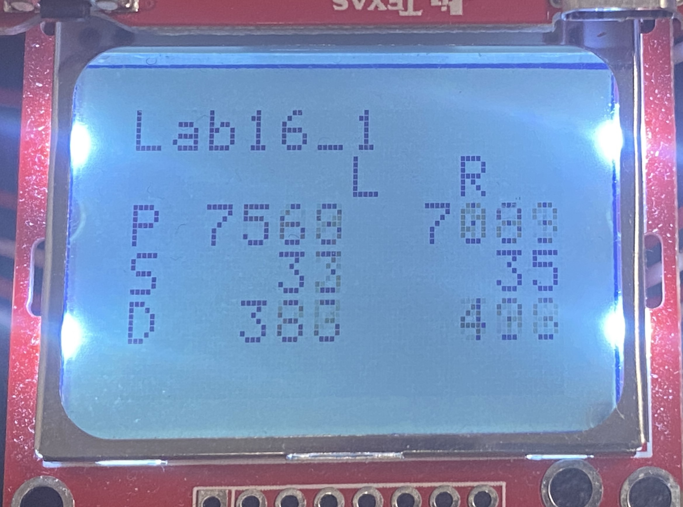
Demo
Program16_1()running at the speeds of 20%, 40%, 60%, 80%, and then return to 20% as shown below.
Video Credit: C26 Peter Choi, Royal Military College of Canada
Graph duty cycle versus actual speed.#
Program16_1()stores the speed of each motor and their corresponding duty cycles in the following buffers.uint16_t SpeedBufferL[BUFFER_SIZE]; // Buffer to store left motor speed data uint16_t SpeedBufferR[BUFFER_SIZE]; // Buffer to store right motor speed data uint16_t DistanceBufferL[BUFFER_SIZE]; // Buffer to store left motor distance data uint16_t DistanceBufferR[BUFFER_SIZE]; // Buffer to store right motor distance data uint16_t DutyBuffer[BUFFER_SIZE]; // Buffer to store duty cycle values
Upon completion of of
Program16_1, the LCD will display an option to transmit the data stored in the buffers, as illustrated below.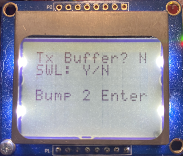
Press the left switch to select “Y” (yes), but do not press any bump switch yet.
Connect the USB cable to the robot and open a serial terminal, following the steps outlined in Lab 11.
When you’re ready to transmit data to the serial terminal, press one of the bump switches. The data will be transmitted as shown below.
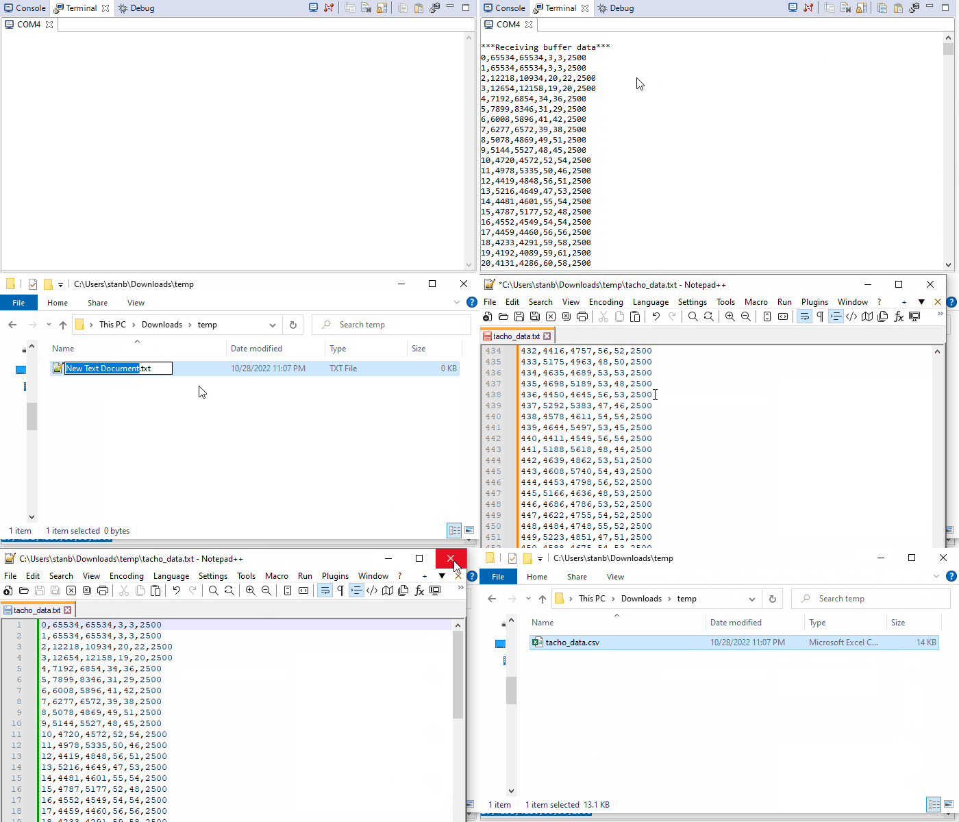
Once the data transmission is finished, the LCD will indicate
TX is Done.In the serial terminal, select the entire data, excluding the header, which reads Receiving buffer data.
Copy the selected data and save it as a text file with a .txt extension or as a comma-separated value (CSV) file with a .csv extension.
Use a software tool of your choice to create plots for the duty cycle in percent, speeds in rpm, and displacement in mm using data from the
SpeedBuffer,DistanceBuffer, andDutyBufferarrays. Recommended software tools include, but are not limited to, MATLAB, Excel, Python with matplotlib, and Jupyter notebook. You can also utilize the Jupyter notebook in Colabused for Lab 15
It is crucial to emphasize that data-driven analyses are fundamental in engineering and scientific endeavors. While videos and images can be helpful for showcasing work, they should never replace the core elements of engineering experiments. Collecting accurate measurements, creating informative plots, and conducting comprehensive analyses will be essential to your final presentations and reports.
Caution
Full credit will only be awarded if the figures include correct labels and units. You must use standard units. Units such as permille or 10 ms are not considered standard, whereas RPM, percent, and milliseconds are acceptable.
Ensure that the first column of the data represents time in 10-millisecond intervals; “1” signifies 10 ms, and “2” signifies 20 ms.
Label your axes with appropriate units, e.g.,
time (seconds)ortime (ms). Convert the time data from 10 ms to seconds or milliseconds. You have to use standard units, such as seconds (sec), milliseconds (ms), and microseconds (us). Note that 10 ms is not a standard unit of time. Therefore, it is essential to convert the time data into seconds (sec) or milliseconds (ms), and you should be familiar with the process of converting from 10 ms to seconds (or ms).Represent the duty cycle in
percentagerather thanpermillesincepermilleis not a standard unit.Express the speed in rpm, rotations per minute (RPM).
Examples of incorrectly labeled plots include, but are not limited to, the following.
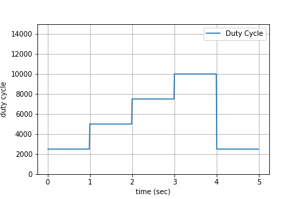
The y-axis in this plot is incorrect; it lacks units, and the correct standard unit for the duty cycle is percent.
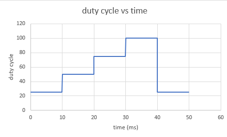
The x-axis in this plot is incorrect; it should span from 0 to 5 seconds. Additionally, the entire transition cannot be completed within just 50 milliseconds. This suggests that the plot was not carefully reviewed before submission, which is unacceptable in the field of engineering. You will be very likely to receive no credit for such a plot as it clearly demonstrates a fundamental misunderstanding of what the data represents. It’s akin to claiming that the power efficiency in your analysis is 120% or -5% — an obvious and critical error.
Submit the following plots on Gradescope.
Distances vs. time
Speeds vs. time
Duty cycle vs. time
Finite State Machine#
Note
This part is the foundation of Deliverable 1 of the final project.
Complete
Controller3to implement the finite state machine as shown below.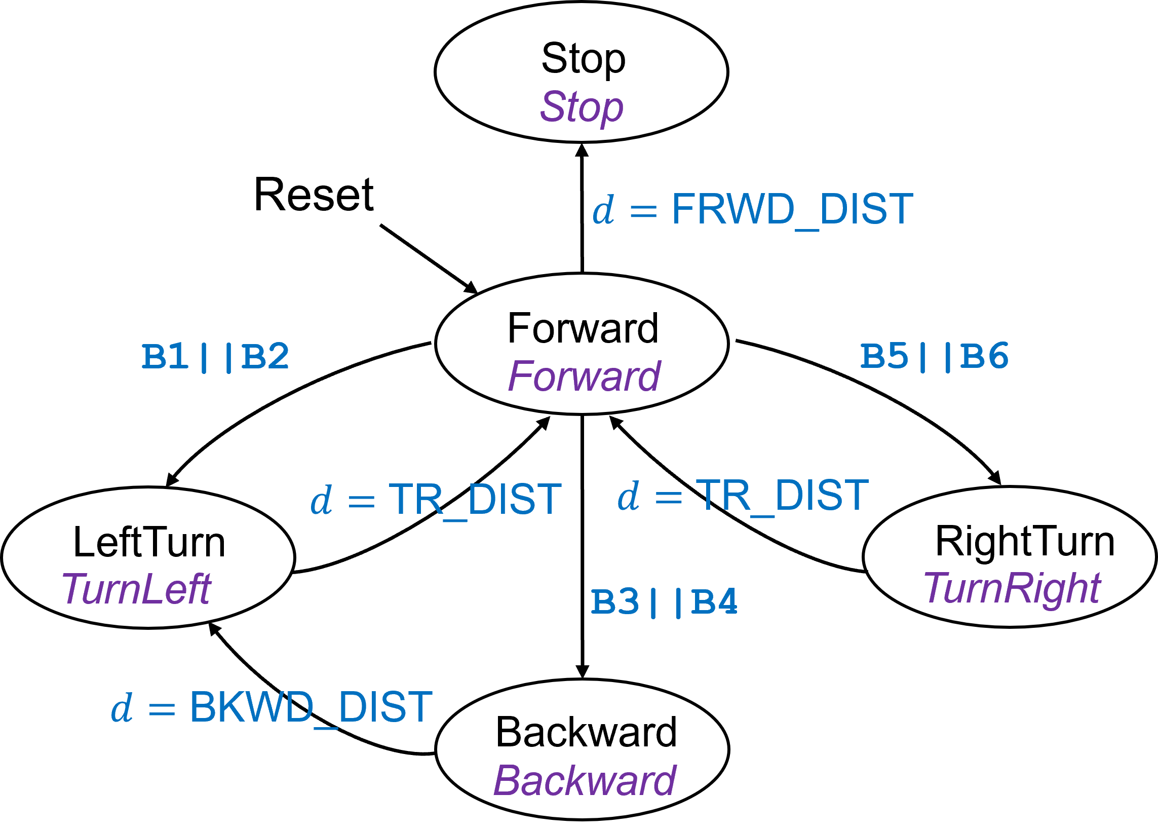
FRWD_DIST = 700 mm.
BKWD_DIST = 90 mm.
TR_DIST refers to the displacement for a 30\(^\circ\), 60\(^\circ\), or 90\(^\circ\) turn depending on the bump switch triggered.
Start in the Forward state.
If Bump3 or Bump4 is triggered, move backward 90 mm, make a 90\(^\circ\) left turn, and then move forward.
If Bump1 is triggered, make a 30° left turn, then move forward.
If Bump2 is triggered, make a 60° left turn, then move forward.
If Bump5 is triggered, make a 60° right turn, then move forward.
If Bump6 is triggered, make a 30° right turn, then move forward.
If no bump switch is triggered while in the Forward state, move forward for 700 mm and then stop.
Ignore any bump triggers in states other than Forward,
Demo
Program16_3to showcase the finite state machine by running your robot on the floor.
🚚 Deliverables#
Deliverable 1#
[9 Points] Demo
Program16_1()running at the speeds of 20%, 40%, 60%, 80%, and then return to 20%.
Deliverable 2#
[8 points] Use a software tool of your choice to create plots for the
duty cycle in percent,timer periods in microsecond, andactual speeds in rpm. Submit your three plots in Gradescope.
Deliverable 3#
[9 Points] Demo
Program16_3()to showcase the finite state machine by running your robot on the floor.
Deliverable 4#
[8.5 Points] Ensure that you provide comments in your code for clarity and push your code to your repository using git.
This lab was originally adapted from the TI-RSLK MAX Solderless Maze Edition Curriculum and has since been significantly modified.
