🔬 Lab 17 Control Systems#
📌 Objectives#
Students should be able to integrate input capture measurements from Timer A3 and PWM outputs using Timer A0.
Students should be able to design and implement a speed control system for dual motors.
Students should be able to assess the effectiveness and performance of the control system.
Students should be able to develop a proportional controller for a wall-following robot.
Note
If debugging is the process of removing software bugs, then programming must be the process of putting them in. -Edsger Dijkstra
📜 Synopsis#
Equipped with the knowledge gained from previous labs, we now have the tools to both drive the robot and gather data on various parameters, including the robot’s speed, distance traveled, and the distance to nearby walls. In this lab, our focus will be on implementing automatic controllers that enable the robot to perform specific tasks, such as driving between walls. These control methods belong to the category known as proportional-integral-derivative (PID) control systems.
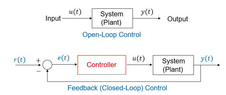
If the controller does not utilize feedback from the system’s output to compute the control action, it is referred to as an open-loop control system. Conversely, when the system’s output is measured and used as feedback in the controller’s computation, it is termed a closed-loop or feedback control system. The diagram below illustrates both open-loop control (top) and closed-loop control (bottom) systems.

Note
Control systems are a rich, complex field within engineering, spanning electrical, robotics, aerospace, mechanical, and computer engineering. This module provides an introductory overview.
💻 Procedure#
Setup#
Naviate to ECE382 Teams > General > Files > Class Materials > SourceFiles.
Download
Program17_1.candProgram17_3.c, and place them in theLab17_Controlfolder to replace the existing files. They must be located in the project folder, not in theincfolder.
Implement a proportional-integral controller in Program17_1#
This is part of Homework 17
Read
Program17_1.cthoroughly. A solid understanding of the code will reduce the time needed for both this assignment and the final project.Complete the
Controller()function inProgram17_1.cfollowing the provided instructions.Implement a proportional-integral controller to control both motors at the desired speed.
Copy your
Controller()code into Gradescope for Homework 17 submission.
Demo Program17_1#
Experimentally determine the best \(K_p\) and \(K_i\) to achieve a stable system.
Adjust \(K_p\) and \(K_i\), which are defined at the beginning of
Program17_1.c. You can also fine-tune these values in real-time using the bump switches.Note that the average PWM introduced on Lecture 17, Slide 14 is designed for the wall-following robot and should not be used here, as it may reduce the controller robustness.
Record the \(K_p\) and \(K_i\) values and report them in the following section.
Demonstrate the functionality of
Program17_1()with a proportional-integral controller that maintains wheel speeds of 50 rpm and 100 rpm despite external disturbance. Be sure to apply the disturbance only after the desired speed has settled. To test the disturbance rejection, apply light friction to the wheels as shown in the video below.
Discuss the performance of your controller in Program17_1()#
Gather wheel speed data at 100 rpm through the USB/UART port and evaluate the performance in
Program17_1().You may need to adjust the Serial Terminal buffer size, which defaults to 1000 lines. If you require more than 1000 lines, refer to the instructions here.
Provide the step response of the speed controller with an external disturbance, ensuring that disturbance is applied after the speed has settled at the desired speed.
Provide the input signals (PWM duty cycles) applied to the robot.
Feel free to use any software of your choice, such as MATLAB or MS Excel, to generate figures. Ensure your plots include labels, units, and legends as needed. Make sure to focus on the region of interest and utilize axis limit functions like
plt.ylimorplt.xlim.Discuss the controller’s performance in terms of response time, overshoot, and steady-state error. Report the \(K_p\) and \(K_i\) values used for these plots.
Analyze your controller’s disturbance rejection using the plots.
Warning
Take this part very seriously. The critical component of your final report will involve analyzing the system’s performance. Scientific analysis predominantly relies on the data gathered, frequently presented through figures.
This analysis section holds nearly twice the points as the demonstration
Examples of plots that may not receive full credit include, but are not limited to, the following.

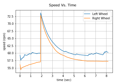
The above plot has no step response. The initial motor speeds must be 0.

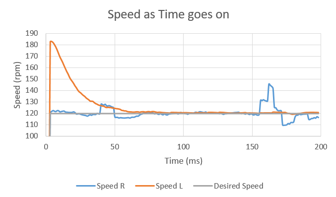
The x-axis is off by at least an order of magnitude. The whees cannot react at the speed shown in the plot.

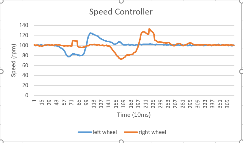
The x-axis unit should be in seconds (s) or milliseconds (ms), not 10 ms or 20 ms. The standard time units in engineering are s, ms, us, ns, and so on.
Implement a Wall-Following controller in Program17_3#
Complete the
Controller()function inProgram17_3.c.Develop a proportional controller to steer the robot between two walls using IR sensors.
Experimentally find the optimal proportional constant and swing values to achieve a stable system.
Determine three distinct \(K_p\) values for the following responses:
Slow response
Fast response with minimum or no overshoot
Very fast response with significant overshoot.
Document the \(K_p\) values in the report section.
Demo
Program17_3using the three \(K_p\) values. Important Note: Start the robot at least 3 inches (or 7.5 cm) from the center line, with one wheel on the white center line.
Evaluate controller performance in Program17_3()#
Collect data via the USB/UART port to assess the controller’s performance.
Provide the step response of the closed-loop system for a fast response with a slight or no overshoot, identified in Deliverable 3. The step response should show the system’s output, i.e., distance from the center.
Plot the input signal associated with this step response. The input signal applied to the system is the PWM duty cycles in percent.
Report the \(K_p\) value associate with these plots. 1.Utilize software of your choice, such as MATLAB or MS Excel, for generating figures. Ensure that your plots feature labels, units, and legends when necessary. Evaluate controller performance in terms of response time, overshoot, and steady-state error.
This analysis section also carries nearly twice the points as the demonstration.
🚚 Deliverables#
Deliverable 1 [5 Points]#
Demonstrate the functionality of
Program17_1()with a proportional-integral controller for regulating wheel speeds at 50 rpm and 100 rpm, ensuring disturbances are applied only after the speed has stabilized.
Deliverable 2 [9 Points]#
Provide a step response of the speed controller with a disturbance, applied after the speed settles at the desired speed. Include plots with labels, units, and legends as needed.
Provide the input signals (PWM duty cycles) applied to the robot.
Discuss the controller’s performance in terms of response time, overshoot, and steady-state error. Report the \(K_p\) and \(K_i\) values used for these plots.
Analyze your controller’s disturbance rejection using the plots.
Deliverable 3 [5 Points]#
Demo
Program17_3using the three different \(K_p\) values. Important Note: Ensure that your robot is initially positioned at least 3 inches (or 7.5 cm) away from the center line. Your demo must include three step responses: slow response, fast response with minimal overshoot, and very fast response with significant overshoot. Report their \(K_p\) values.
Deliverable 4 [9 Points]#
Collect data via the USB/UART port to assess the controller’s performance. Provide the \(K_p\) values recorded in the previous section. Provide the best step response from Deliverable 3, along with the input signal (PWM duty cycles) applied to the robot. Report the corresponding \(K_p\) value. Evaluate the controller’s performance based on response time, overshoot, and steady-state error.
Deliverable 5#
[6.5 Points] Ensure that you provide comments in your code for clarity and push your code to your repository using git.
This lab was originally adapted from the TI-RSLK MAX Solderless Maze Edition Curriculum and has since been significantly modified.
