Lesson 8 – Circuits 4: AC Circuit Analysis

Learning Outcomes

1. Articulate the difference between DC and AC signals.

2. Draw the graph of a cosine, labeling its amplitude and its period.

3. Derive the equation of a cosine from its graph.

4. Apply KVL, KCL, and Ohm’s Law to AC-powered resistive circuits.

5. Calculate the RMS value (current or voltage) of an AC signal.

6. Explain what the RMS value means and how it relates to a DC value.

7. Calculate the average power produced or consumed in an AC circuit.

Electrical Signals

Our world is filled with signals. We raise our hand to signal the instructor when we know the answer to a question. The light turns red to signal we should stop. The phone rings to signal we should answer it. Generally, a signal is something that conveys information.

In the world of electrical engineering, we use signals to convey information and transmit power. The TV signal that comes to our homes via cable, satellite dish, or old-fashioned antenna, is an electrical signal that contains video images and the sound that goes with them. When we click our mouse, an electrical signal is processed by our computer’s microprocessor to tell the correct program what to do. In our combat aircraft, electrical signals are used to release bombs and missiles at the proper time to cause the most damage to our adversaries. Our communication systems use electrical signals to link weapon systems and warfighters, thereby maintaining battlefield situational awareness. Our power grid uses a very specific signal to transmit power efficiently over long distances.

In the previous lessons, we examined how an electrical signal may be used to deliver power to a load, such as a light bulb, and in doing so, we used voltage sources that always provided the same voltage to the circuit. However, in this lesson, we will introduce a voltage source that can change its voltage over time. This new voltage source will allow us to send different electrical signals to our load in order to transmit power or convey information. This lesson will focus on using these new electrical signals to transmit power, while blocks 3 and 4 will focus on how these signals may be used to convey information.

Example Problem 1

A programmable laser pointer is modeled as the following circuit. Graph the current provided by the voltage source as a signal with respect to time.

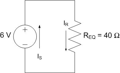
Fig. 2. Circuit for Example Problem 1: 1.5 V source powering a laser pointer modeled with R_1 (50 Ω) in series with R_2 and R_3 (500 Ω each) in parallel.

Understand: This is a review of material from the last lesson. We have a source connected to a load, which consists of multiple resistors in both series and parallel.

Identify Key Information:

• Knowns: \(V_S\) = 1.5 V, and the resistances in the load.

• Unknowns: \(R_{EQ}\) and \(I_S\).

• Assumptions: The source provides all the current needed by the load.

Plan: Calculate the equivalent resistance, then use Ohm’s Law to find the source current.

Solve: \(R_2\) and \(R_3\) are connected in parallel:

\[R_{23} = \frac{(500\ \Omega)(500\ \Omega)}{(500\ \Omega) + (500\ \Omega)} = 250\ \Omega\]

This 250-Ω resistor is in series with \(R_1\):

\[R_{EQ} = R_{1} + R_{23} = 50\ \Omega + 250\ \Omega = 300\ \Omega\]

Fig. 3. Equivalent circuit for Example Problem 1: 1.5 V source with a single 300 Ω equivalent resistance.

\[I_{S} = \frac{V_{S}}{R_{EQ}} = \frac{1.5\ \text{V}}{300\ \Omega} = 5\ \text{mA}\]

Answer: Since there is nothing in the circuit to make the current change over time, the graph of the current signal is a flat line at 5 mA — a DC signal.

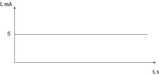
Fig. 4. DC current signal for Example Problem 1: a flat line at 5 mA, constant for all time.

A DC (Direct Current) signal does not change over time; its voltage and current stay the same for all time.

AC Signals

On the other hand, AC signals are more interesting to examine since they vary with time. Frequently, AC signals are sinusoidal; therefore, we use the following standard equation form to describe them:

Key Concept — AC Signal Standard Form

\[v(t) = V_{Bias} + V_{m}\cos(360^\circ \cdot f \cdot t - \phi)\ \text{V}\]

\(V_{Bias}\): DC component (average value)   \(V_m\): amplitude   \(f\): frequency (Hz)   \(\phi\): phase shift

This standard format is portrayed graphically in Figure 1.

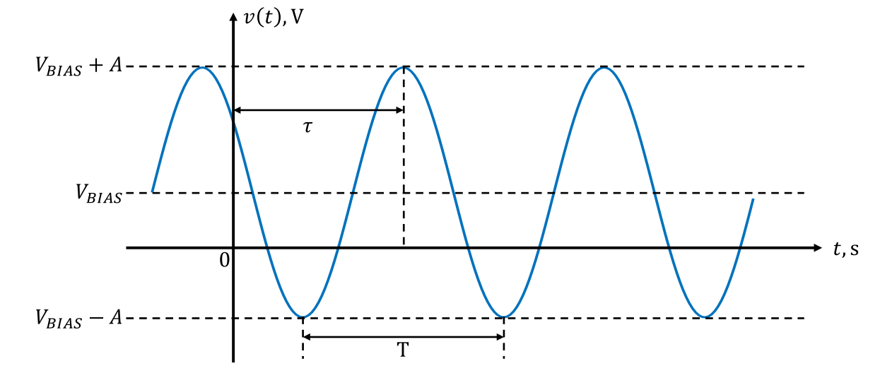
Fig. 1. Graphical representation of the AC standard form.

In order to graph the signal, we must introduce two more parameters. First, the period of the signal, T, is the time the signal takes to complete a cycle:

Key Concept — Period and Time Delay

\[T = \frac{1}{f} \qquad \tau = T\frac{\phi}{360^\circ}\]

\(T\): period (time to complete one cycle)   \(\tau\): time delay (time shift of the peak from \(t = 0\))

We will also use the same format for current by replacing \(v(t)\) with \(i(t)\), \(V_{Bias}\) with \(I_{Bias}\), and volts with amps.

Additionally, when we know the maximum and minimum values of a signal, we can solve for the bias and amplitude using:

Key Concept — Bias and Amplitude from Max/Min

\[V_{Bias} = \frac{v_{max} + v_{min}}{2} \qquad V_{m} = \frac{v_{max} - v_{min}}{2}\]

Example Problem 2

A building is wired with AC power with a voltage of \(v_s(t) = 170\cos(360^\circ \cdot 60\ \text{Hz} \cdot t)\ \text{V}\). If two 200-Ω light bulbs are connected in parallel to this source, graph the signal of the current drawn from the source.

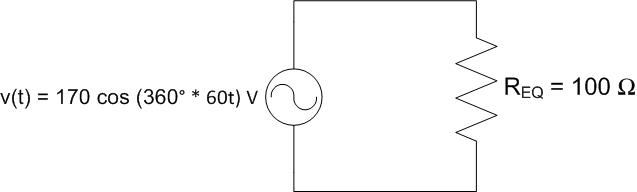
Fig. 5. Circuit for Example Problem 2: AC voltage source \(v_s(t) = 170\cos(360° \cdot 60\ \text{Hz} \cdot t)\ \text{V}\) powering two 200 Ω bulbs in parallel.

Understand: Although we are dealing with a sinusoidal input signal, all of the rules we’ve learned for resistive circuits still apply. We can solve this problem by finding the equivalent resistance and using Ohm’s Law.

Identify:

• Knowns: \(v(t) = 170\cos(360^\circ \cdot 60\ \text{Hz} \cdot t)\ \text{V}\); two 200-Ω bulbs in parallel.

• Unknowns: The source current \(i_s(t)\).

• Assumptions: Our tools for analyzing resistive circuits still apply.

Plan: Find the equivalent resistance, then use Ohm’s Law to find \(i_s(t)\). Use the standard equation to draw the graph.

Solve:

\[R_{EQ} = \frac{(200\ \Omega)(200\ \Omega)}{(200\ \Omega) + (200\ \Omega)} = 100\ \Omega\]

Since the two devices are in parallel, all the source voltage drops across \(R_{EQ}\):

\[i_s(t) = \frac{v_s(t)}{R_{EQ}} = \frac{170\cos(360^\circ \cdot 60\ \text{Hz} \cdot t)}{100\ \Omega} = 1.70\cos(360^\circ \cdot 60\ \text{Hz} \cdot t)\ \text{A}\]

The amplitude is 1.70 A. The frequency is 60 Hz, so the period is:

\[T = \frac{1}{60\ \text{Hz}} = 16.67\ \text{ms}\]

Answer: The graph of the source current signal is:

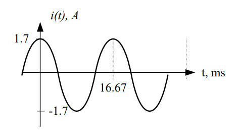
Fig. 6. AC current signal for Example Problem 2: \(i_s(t) = 1.70\cos(360° \cdot 60\ \text{Hz} \cdot t)\ \text{A}\), amplitude 1.70 A, period 16.67 ms.

AC Power

The concept of power for AC signals can be difficult to understand because the voltages and currents are constantly changing, meaning the power is always changing as well. If we simply take the voltage across and the current through a device and multiply them together, we get something known as instantaneous power:

\[p(t) = i(t)\ v(t)\]

For our example above, we can see that the power of an AC signal varies over time and even drops to 0 W at regular intervals. What we want is a way to measure the average power.

We can’t simply multiply the average voltage by the average current to get average power. Doing this would result in 0 W because the average voltage and current for a pure AC signal are both zero. Instead, we introduce the root-mean-square (RMS) value. The RMS value represents the magnitude of the equivalent DC voltage (or current) that would dissipate the same amount of power in a resistor.

For sinusoidal signals:

Key Concept — RMS Value and Average Power

\[V_{RMS} = \sqrt{(V_{Bias})^{2} + \frac{(V_{m})^{2}}{2}}\]

For zero-bias signals: \(\displaystyle V_{RMS} = \frac{V_m}{\sqrt{2}}\)

\[P_{AVG} = I_{RMS} V_{RMS}\]

So for the example above (\(V_m\) = 170 V, \(I_m\) = 1.70 A):

\[V_{RMS} = \frac{170}{\sqrt{2}} = 120.2\ \text{V}_{RMS}\]

\[I_{RMS} = \frac{1.70}{\sqrt{2}} = 1.202\ \text{A}_{RMS}\]

\[P_{AVG} = I_{RMS}V_{RMS} = 144.5\ \text{W}\]

The voltage used here has a frequency of 60 Hz and a voltage of 120 \(V_{RMS}\) — exactly the voltage we get out of our wall outlets in the United States. When we say the wall outlet gives us 120 volts, what we really mean is that it gives 120 volts RMS. The actual signal varies from 170 V to −170 V at 60 Hz.

Key Takeaways

• DC vs. AC Signals. A DC (Direct Current) signal has a constant voltage and current for all time, while an AC (Alternating Current) signal varies sinusoidally and can be described by amplitude, frequency, bias, and phase shift.

• AC Standard Form. Sinusoidal signals are written as \(v(t) = V_{Bias} + V_m\cos(360° \cdot f \cdot t - \phi)\), where each parameter has a direct graphical interpretation.

• Period and Frequency. The period T = 1/f is the time for one complete cycle; frequency f is measured in hertz (Hz) and determines how rapidly the signal oscillates.

• Bias and Amplitude. The DC bias is the average value of the signal (\(V_{Bias} = (v_{max}+v_{min})/2\)) and the amplitude is half the peak-to-peak swing (\(V_m = (v_{max}-v_{min})/2\)).

• Ohm’s Law for AC Circuits. KVL, KCL, and Ohm’s Law apply to AC resistive circuits the same way they apply to DC circuits; the result is a sinusoidal current with the same frequency as the source.

• RMS Value. The root-mean-square voltage or current represents the equivalent DC value that delivers the same average power; for a zero-bias sinusoid, \(V_{RMS} = V_m / \sqrt{2}\).

• Average AC Power. Average power in an AC resistive circuit is calculated as \(P_{AVG} = I_{RMS} V_{RMS}\); the US standard outlet delivers 120 V\(_{RMS}\) at 60 Hz, corresponding to a peak voltage of approximately 170 V.