Lesson 30 – Demodulation

Learning Outcomes

1. Compute transmitter power efficiency for an AM system with a given modulation index.

2. Describe block diagram AM demodulators and their limitations.

3. Analyze envelope detectors in the time domain and synchronous detectors in the frequency domain.

4. Given an AM modulated signal, design an AM demodulator to recover the original message.

5. Explain the engineering trade-offs between over- and under-modulated AM communication scenarios.

---

Demodulation

The last several lessons have focused on modulation. This lesson focuses on demodulating signals to recover the original information and understanding the associated trade-offs.

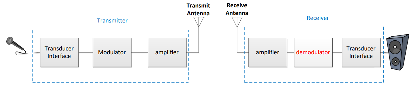
Fig. 1. Overview of a communications system showing where demodulation fits: the receiver recovers the original message from the modulated carrier.

---

Modulation Efficiency

Previously, we introduced adding a bias signal before modulation. As bias increases, time-domain envelopes separate and a carrier spike appears in the frequency domain.

Two AM types:

• DSB-SC: Information in sidebands only

• DSB-LC: Information in sidebands + carrier

Over-modulated	100%-modulated	Under-modulated
\(\alpha \rightarrow \infty\)	\(\alpha = 1\)	\(\alpha = 0.667\)

Efficiency is defined as:

\[ \eta = \frac{\text{useful power}}{\text{total power}} = \frac{P_{USB} + P_{LSB}}{P_{total}} \]

Power:

\[ P = \frac{V_{rms}^2}{R}, \quad V_{rms} = \frac{V_m}{\sqrt{2}}, \quad P = \frac{V_m^2}{2R} \]

With normalized resistance \(R = 1\ \Omega\):

Key Concept — AM Modulation Efficiency

\[\eta = \frac{\alpha^2}{\alpha^2 + 2}\]

• DSB-SC: \(\eta = 100\%\)

• \(\alpha = 1 \Rightarrow \eta = 0.33\)

---

Envelope Detector

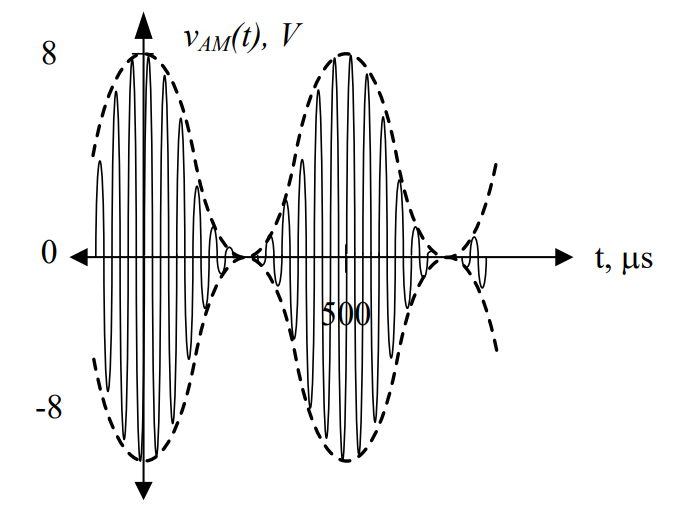
Under-modulated signals allow envelope detection.

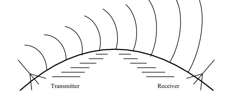
Fig. 2. Envelope detector block diagram: diode (rectification) → LPF (removes carrier) → HPF (removes bias) → recovered message.

Steps:

1. Diode (rectification): Removes negative portion

2. LPF: Removes carrier

3. HPF: Removes bias

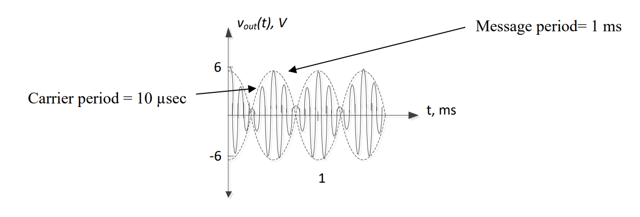
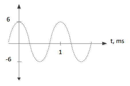
Fig. 3. Signal at each stage of the envelope detector: AM input → rectified (diode) → smoothed (LPF) → DC removed (HPF) → message output.

---

Example Problem 1

Understand: Under-modulated → envelope detector works.

Identify Key Information:

• Known: \(T_M = 250\ \mu s\)

• Unknown: carrier

Plan: Define LPF and HPF cutoff frequencies.

Solve:

\[ f_M = \frac{1}{T_M} = \frac{1}{250\ \mu s} = 4\ kHz \]

• LPF cutoff \(> 4\ kHz\)

• HPF cutoff \(> 0\ Hz\) (use 10 Hz)

---

Envelope Detector Components and Rules

• Diode: removes negative voltages

• LPF: removes carrier

• HPF: removes bias

Rules:

• \(f_{LPF} > f_{m,\ max}\)

• \(f_{HPF} > 0\)

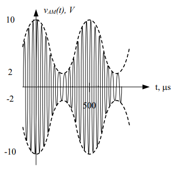
Envelope detectors do not work for:

• Over-modulated signals

• DSB-SC

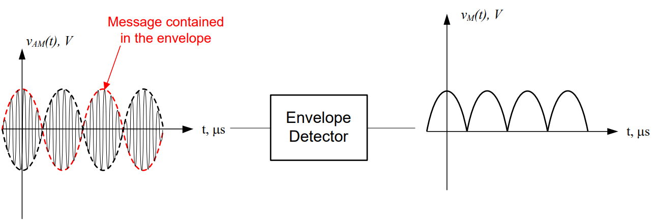
Fig. 4. Envelope detectors only work for under-modulated signals — over-modulated signals and DSB-SC cannot be recovered this way.

---

Synchronous Detector

Used for all modulation types.

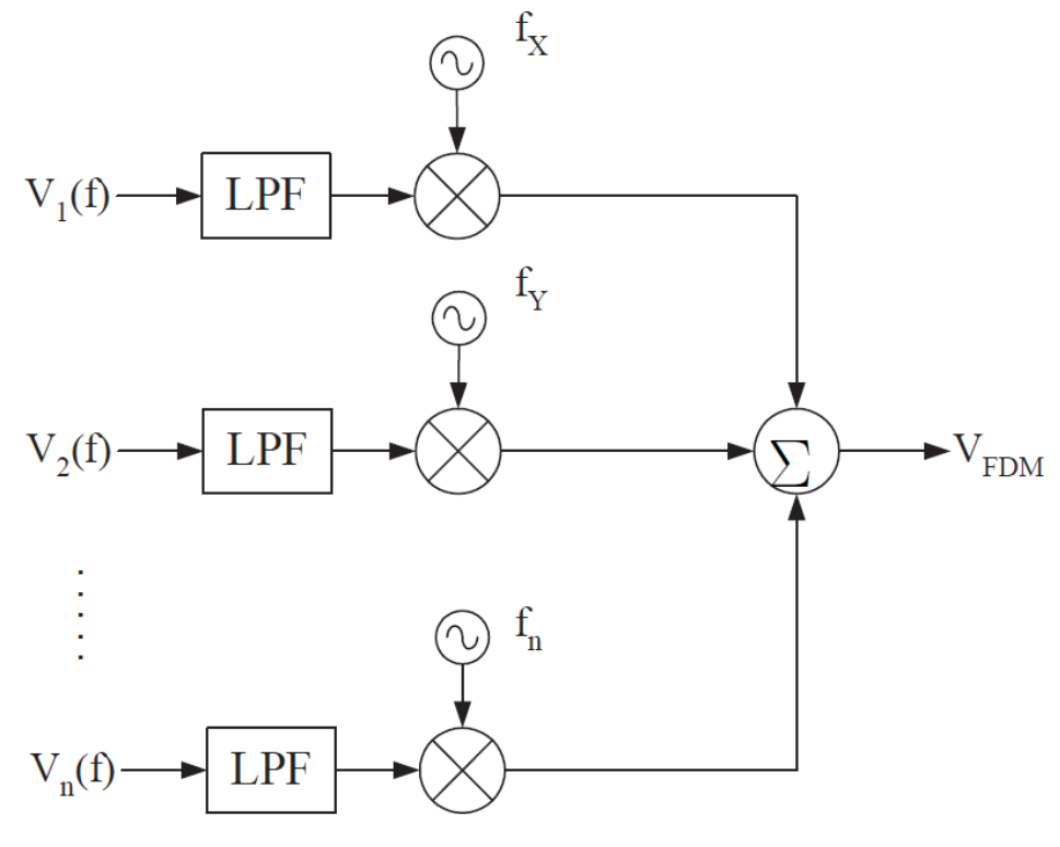
Fig. 5. Synchronous detector block diagram: modulated input is multiplied by the carrier frequency, then filtered to recover the message.

Multiply by carrier frequency:

• Shift up: \(f + f_c\)

• Shift down: \(f - f_c\)

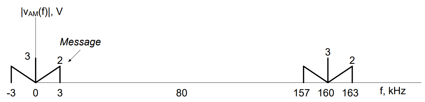
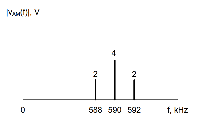
Fig. 6. Frequency shift after multiplying by carrier: sidebands shift up to \(f + f_c\) and down to \(f - f_c\), producing components at baseband and double-carrier frequencies.

Negative frequencies reflect and double amplitude.

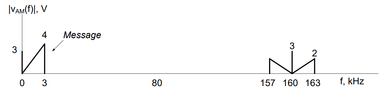
Fig. 7. Spectrum after reflecting negative frequencies: amplitudes at baseband double; the LPF then removes the high-frequency components.

Apply LPF:

• Choose \(f_{LPF} > f_{m,\ max}\)

Then HPF:

• Remove DC bias

---

Final Design

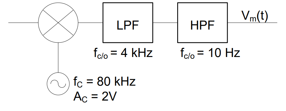
Fig. 8. Final synchronous demodulator design: multiplier (carrier frequency) → LPF (\(f_{LPF} \geq f_{m,\max}\)) → HPF (removes bias) → recovered message.

Components

• Multiplier: shifts to baseband

• LPF: removes high-frequency content

• HPF: removes bias

Design Rules

• Demodulating frequency = carrier frequency

• \(f_{LPF} \ge f_{m,\ max}\)

• \(f_{HPF} > 0\) (≈ 10 Hz)

Key Takeaways

• Demodulation goal. Recover the original message signal from the received AM waveform by reversing the modulation process.

• AM efficiency (\(\eta\)). The fraction of transmitted power that carries useful information; a lower modulation index wastes more power on the carrier and reduces efficiency.

• Envelope detector. A simple circuit (diode → LPF → HPF) that recovers the message by following the amplitude envelope of the AM signal; only works when the modulation index \(\alpha \leq 1\).

• Over-modulation failure. When \(\alpha > 1\) the carrier inverts during negative message peaks, causing the envelope detector to produce a distorted output — a synchronous detector must be used instead.

• Synchronous (product) detector. Multiplies the received signal by a locally-generated carrier copy, shifting the sidebands back to baseband, then uses an LPF and HPF to extract the message; works for all modulation types and all modulation indices.

• LPF cutoff rule. The low-pass filter must have \(f_{LPF} \geq f_{m,\max}\) to pass the full message bandwidth without cutting off high-frequency message components.

• HPF role. The high-pass filter (with \(f_{HPF} \approx 10\ \text{Hz} > 0\)) removes the DC bias that was added during modulation, leaving only the recovered message signal.