Lesson 24 – Analog-to-Digital Conversion 1#
Learning Outcomes
Compare and contrast the advantages and disadvantages of digital signals.
Define sampling rate in an analog-to-digital converter (ADC) and articulate its engineering impacts.
Calculate the resolution of an ADC and articulate its engineering impacts.
Given a voltage input to an ADC, and its operational parameters (sampling rate, dynamic range, and number of output bits), determine the digital output.
Analog to Digital Conversion#
As humans, we use analog senses to perceive the world. Our eyes detect subtle variations in the color and intensity of light. Our ears discriminate between a wide and continuous range of frequencies and sound levels. Our senses of taste, touch, and smell also differentiate between a continuous range of inputs. By definition, analog values are continuous, where they can have any value between a defined maximum and minimum value at any given instant in time. For example, our eyes perceive infinite shades of gray—this is analog. Digital means we only allow for a signal to be expressed in terms of values from a certain predetermined set of values. It would be akin to seeing the world in only black and white, or perhaps only specific combinations of red, green, and blue. Either way, we are restricting the possible values of our signal.
One special type of digital value is called binary, which only allows two possible values. Computers (and many things we call digital) use binary values to store and transmit information.
A huge amount of Electrical and Computer Engineering is spent bridging the gap between the physical world’s analog information and digital technology. Consider all the technologies which have been digitized over the last 15 years—cameras, cell phone communications, and TVs are just a few examples. What drove us to convert these technologies to digital?
Digital is less susceptible to noise, which is the static that you hear in older radios and cell phones.
Digital can be easily stored and recovered, because the amount of data is significantly reduced.
Digital allows for easier encryption and processing by computers.
Digital signals have disadvantages, which is why many technologies start off with analog implementations. For example, the original version of the modern day computer was analog. When you convert your original analog information into a digital format, you lose some fidelity of the information. There’s no way to go from a continuous range of infinite values to discrete levels without throwing something away. Although we can minimize information loss by increasing the number of possible discrete values, this also increases the amount of digital information that you have to save, process, and transmit. For example, an image from a 12 megapixel (MP) camera is a significantly larger file size than a photo from a 1 MP camera.
As we discuss the process of converting data from analog to digital, hopefully you’ll begin to understand the tradeoffs. Digitizing a signal consists of three basic steps: sampling, quantizing, and encoding.
Sampling#
Sampling an analog signal means taking a set number of measurements each second. The rate at which we take these measurements, or the sampling rate, is simply how often we take a snapshot of whatever it is we’re trying to sample within a second. Think about watching a show on TV. Even though the movement on the screen looks fairly natural, it really has a sampling rate of 60 frames per second, or 60 Hz. Every \(1/60\) of a second, the TV’s screen updates. In fact, if you take a slow motion video of your TV with your camera, you will see the flickering of the screen, which is the update rate. This is actually the fact that a slow motion video is taking many more samples per second than the TV, so it “sees” the update rate of the screen.
But what if our TV only updated once per second—would that be enough? What about 1 update per minute? Obviously, there is some minimum standard for how often we need to sample whatever we’re trying to digitize. The limit is based on the Nyquist rate, which is simply two times the highest frequency in the signal:
Nyquist Sampling Rate
If we sample at a frequency below the Nyquist rate, we get a distortion in the signal known as aliasing. Aliasing is the cardinal sin of ADC—once it occurs, it can’t be fixed. We can correct a lot of problems but aliased data is unrecoverable.
One simple visual example of aliasing is the wheels of a car during a car commercial. Even though the car is obviously moving forward, the wheels sometimes look as if they are rolling backwards. This is because the wheel is spinning at a rate higher than half the Nyquist frequency. For example, consider the wheel of a car spins at a rate of 35 Hz. According to the Nyquist criteria, the required sampling rate would be:
Since the actual TV sampling rate is 60 Hz, the video is aliased and the wheel looks like it is moving backwards. Aliasing can actually change the frequency of the input signal, so that it looks like something completely different. In this case, your digitized signal doesn’t look anything like your analog signal, which defeats the purpose of ADC.
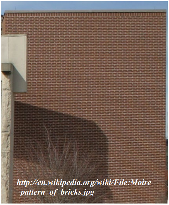
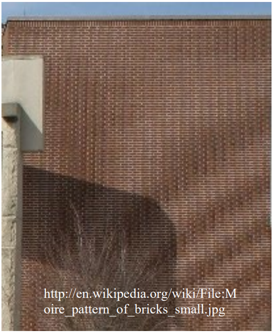
The pictures in Figures 1 and 2 show another example of aliasing. Did you realize that edges in images are a form of high frequency content? The image on the left is sampled well above the Nyquist minimum. When we reduce the number of pixels (or samples), we get aliasing in the form of the pattern in the lower right corner.
|
|
|---|---|
Fig. 1. Properly sampled image. |
Fig. 2. Aliased image. |
Example Problem 1
A typical human voice has a maximum frequency of 3.4 kHz. If we wish to digitize a voice signal, what is the lowest sampling frequency we can use that would prevent aliasing?
Understand: Aliasing is the distortion in a signal when we do not sample it at a high enough rate.
Identify Key Information:
Knowns: The maximum frequency of a human voice and the Nyquist criteria.
Unknowns: The required sampling rate for ADC.
Assumptions: None.
Plan: Sample at least at the Nyquist rate to prevent aliasing.
Solve:
Answer: We must use a sampling rate of at least 6.8 kHz to prevent aliasing.
Now we know we have to sample at a rate greater than the Nyquist rate, but what rate should we use? A good example is music CDs, which are simply digital representations of analog music signals. The human ear has a range between 20 Hz and 22 kHz:
Therefore, CDs need to have a sampling rate at 44 kHz or higher. The actual sampling rate for CDs is 44.1 kHz. But if 44.1 kHz is good, wouldn’t 50 kHz or even 100 kHz be even better? Here, we see the engineering tradeoff. The key is to sample at a high enough frequency to adequately reproduce the signal and a low enough frequency to not exceed our memory capacity or digital bandwidth. For a CD, each sample is stored as a 16-bit binary number (2 bytes). A sampling rate of 44.1 kHz allows up to 80 minutes of uncompressed music to be loaded onto a single disc. While the quality of the music increases slightly with higher sampling rates, it also requires larger discs or reduced play time.
Digitizing#
Now, let’s take a look at how we digitize a signal. Suppose the following sinusoidal signal needs to be converted into a digital signal:
What would the sampled signal look like if we used a 30 kHz sampling frequency? Before we start sampling, we must always check the Nyquist rate to make sure we won’t distort the signal. The Nyquist rate is:
Since the 30 kHz sampling frequency is greater than 6 kHz, we can start taking samples. First, we find the sampling period (the inverse of the sampling frequency):
Therefore, we will take a sample every \(33.33\ \mu\text{s}\). The first three samples are:
Look at Figure 3. With a sampling frequency of 30 kHz, we’ve captured a fairly good representation of the original sinusoidal curve.
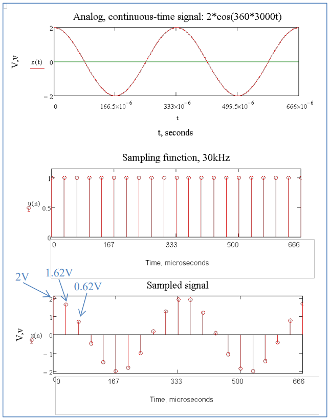
Fig. 3. Sampling \(V_M\).
Resolution#
By virtue of being continuous, analog signals contain an infinite range of magnitude values. Once we have sampled the data, we have reduced the number of values (in time) we need to store. However, we must also convert these values to a finite number of digital outputs (in voltage). After an analog signal is sampled, we must then determine which output to associate with the sampled value. To calculate the discrete level of any given sample, we set voltage limits (\(V_{\max}\) and \(V_{\min}\)) and a number of bits, \(b\), for the process:
The maximum voltage, \(V_{\max}\), is the highest input voltage that will be correctly converted. Input voltages higher than \(V_{\max}\) will be treated as though they were \(V_{\max}\).
The minimum voltage, \(V_{\min}\), is the lowest input voltage that will be correctly converted. Voltages lower than \(V_{\min}\) will be treated as though they were at \(V_{\min}\).
The number of bits, \(b\), that will be used to represent the final digital value determines the total number of possible values:
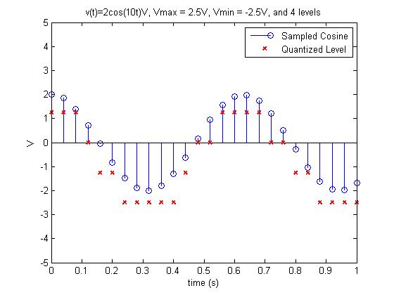
Let’s look at two different settings for converting \(v(t)=2\cos\!\left(360^\circ(1.6\ \text{Hz})t\right)\ \text{V}\). In Figure 5, we allowed each sample to be assigned to one of 16 possible levels, while in Figure 4 we only allowed 4 levels (easier to see the individual levels). Obviously, the levels assigned to each sample in Figure 5 are a truer representation of the original signal.
An important point: the sampling rate and the resolution are completely independent. Sampling divides the signal along the time axis, while resolution divides the signal along the voltage axis.
|
|
|---|---|
Fig. 4. Sampling with 4 levels (\(b=2\) bits). |
Fig. 5. Sampling with 16 levels (\(b=4\) bits). |
Resolution is the smallest voltage change that can be measured by the analog-to-digital conversion process and is equal to:
ADC Resolution
In the examples above, our resolutions were \(1.25\ \text{V/level}\) (Figure 4) and \(312.5\ \text{mV/level}\) (Figure 5). Some important points regarding resolution:
Resolution is determined by the ADC, not necessarily the analog signal being converted. While we want \(V_{\max}\) and \(V_{\min}\) to encompass the range of our input signals, the two ranges are not the same.
A smaller resolution is a better resolution.
The units for resolution are volts per level (V/level).
The range from \(V_{\max}\) to \(V_{\min}\) is called the dynamic range of the ADC. If an input signal exceeds the dynamic range of a particular ADC, it is said to be clipping.
Example Problem 2
A 6-bit ADC has a \(V_{\max}=5\ \text{V}\) and a \(V_{\min}=-1\ \text{V}\). What is the resolution of this ADC?
Understand: The maximum and minimum voltages do not have to be symmetric around 0 V.
Identify Key Information:
Knowns: Dynamic range and number of output bits (\(b=6\)).
Unknowns: Resolution, \(\Delta V\).
Assumptions: None.
Plan: Use the resolution equation:
Solve:
Answer: The resolution is \(93.75\ \text{mV/level}\).
Example Problem 3
An ADC is to be used with \(V_{\max}=4\ \text{V}\) and \(V_{\min}=-2\ \text{V}\). If the worst acceptable resolution is \(200\ \text{mV/level}\), what is the minimum number of bits that can be used?
Understand: More bits \(\Rightarrow\) smaller (better) resolution.
Identify Key Information:
Knowns: Dynamic range and worst acceptable resolution.
Unknowns: Minimum \(b\).
Assumptions: None.
Plan: Solve the resolution equation for \(2^b\):
Solve:
We need \(2^b\ge 30\). Powers of 2: \(2,4,8,16,32\). Since \(32=2^5\), we need \(b=5\) bits.
Using logs:
Rounding up gives \(b=5\).
Answer: 5 bits.
Encoding#
The final step in ADC is to encode the sampled value into a binary number. But first, we must determine what voltage value (or “level”) to assign the sampled value to. Consider the following diagram, where an ADC with 3 output bits is digitizing the signal:
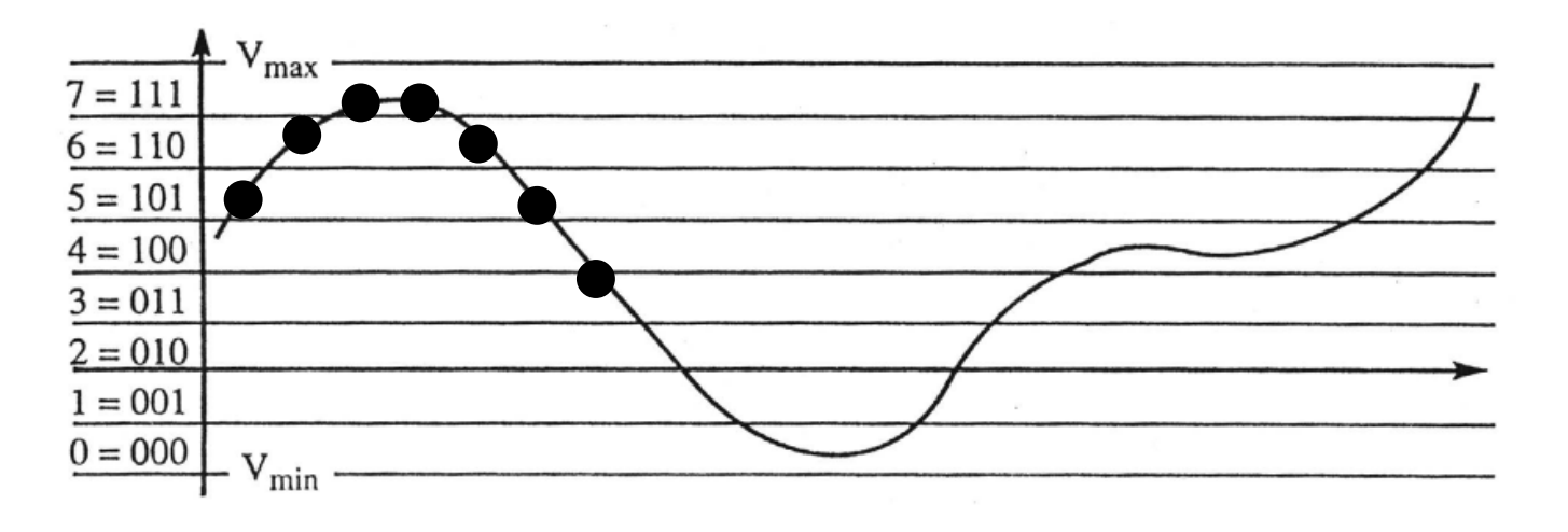
Fig. 6. Example of encoding a signal with a 3-bit ADC.
The black dots represent 7 samples taken from an analog signal. Each level is assigned a number, which is then translated to 3-bit binary. Notice each dot falls into one of the eight levels. The first dot falls into level 5, and therefore is encoded as 101. The second dot is in level 6, or 110. The next two dots are in level 7 (the highest level) and are encoded as 111. The final three dots are in levels 6, 5, and 3 and are encoded as 110, 101, and 011.
If we combine all these samples in series, the binary values resulting from these 7 samples would be:
CD-quality music uses 16 bits per sample. The number of levels is:
Fortunately, there is a simple equation to determine which level a given signal should be assigned:
Expected Level
Once a sample \(V_{in}(t)\) is taken, compute \(EL\) and then round to the nearest integer value. The quantized level is:
Quantization Level
Quantization maps each sample’s continuous voltage to the nearest allowed level (an integer index), and the difference between the true value and the assigned level is the quantization error. For a uniform quantizer with step size ΔV, round-to-nearest bounds this error at half a step:
Quantization Error
We can lower \(\Delta V\) by either:
Reducing the input range (bringing \(V_{\max}\) and \(V_{\min}\) closer), or
Increasing the number of levels (increasing \(b\)).
Often we cannot reduce the range without clipping, so increasing \(b\) is the typical approach—at the cost of more memory and bandwidth.
Putting it All Together#
To convert an analog signal using a specific ADC, you need:
Sampling rate \(f_s\)
Dynamic range \(V_{\max}\) and \(V_{\min}\)
Number of bits \(b\)
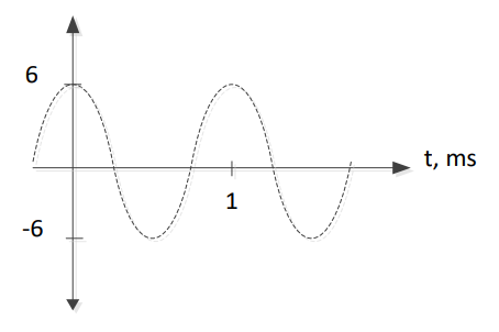
Fig. 7. Overview of the three ADC steps: sampling (time axis), quantizing (voltage axis), and encoding (binary output).
The three steps of analog-to-digital conversion are:
Sampling: Take snapshots in time at the sample rate \(f_s\).
Quantizing: Assign each measured value to one of the available levels.
Encoding: Convert the quantized level into a \(b\)-bit binary number.
Example Problem 4
A sinusoidal signal $\(V_M(t)=2\cos\!\left(360^\circ(3\,\text{kHz})t\right)\ \text{V}\)$ needs to be converted into a digital signal using the following ADC:
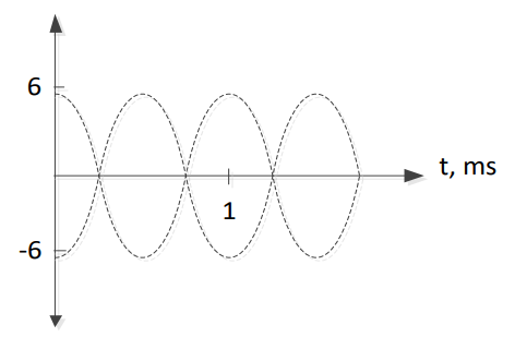
Fig. 8. ADC parameters for Example Problem 4: 5-bit output, \(V_{max} = 3\ \text{V}\), \(V_{min} = -3\ \text{V}\), sampling rate \(f_s = 30\ \text{kHz}\).
Determine the first 3 samples output by the ADC.
Understand: We already have \(f_s\), so now we quantize and encode the samples.
Identify Key Information:
Knowns: Input signal, \(f_s\), number of bits \(b\), and the ADC dynamic range (\(V_{\max}\) and \(V_{\min}\)).
Unknowns: Quantized level and binary code for each sample.
Assumptions: None.
Plan: Compute \(t_s\), evaluate \(V_M\) at sample times, compute \(\Delta V\), compute \(EL\), round to \(QL\), then encode to binary.
Solve:
Sampling period:
Sample times are \(t=n t_s\) for \(n=0,1,2\).
Voltages:
ADC resolution:
Expected levels:
Quantized levels:
Encode to 5-bit binary:
Answer: At \(t=0\), the ADC outputs 11011. At \(t=33.33\ \mu\text{s}\), it outputs 11001. At \(t=66.66\ \mu\text{s}\), it outputs 10011.
Key Takeaways#
Analog vs. digital signals. Analog signals are continuous and can take any value, while digital signals are restricted to a finite set of discrete values; converting to digital reduces noise susceptibility and enables easier storage and processing.
Sampling rate and the Nyquist criterion. The sampling rate \(f_s\) must exceed twice the highest frequency in the signal (\(f_s > 2f_\text{High}\)) to avoid aliasing and faithfully reconstruct the original signal.
Aliasing. When a signal is sampled below the Nyquist rate, aliasing distorts the signal in an unrecoverable way, making the digitized output look nothing like the original.
ADC resolution. Resolution is the smallest voltage change an ADC can distinguish, calculated as \(\Delta V = (V_\text{max} - V_\text{min}) / 2^b\); a smaller \(\Delta V\) means better resolution and finer measurement precision.
Dynamic range and clipping. The range from \(V_\text{min}\) to \(V_\text{max}\) is the ADC’s dynamic range; input signals that exceed this range are clipped and recorded inaccurately at the maximum or minimum output code.
Quantization error. Assigning a sampled voltage to the nearest discrete level introduces rounding error bounded by \(|QE| \le \frac{\Delta V}{2}\); increasing the number of bits \(b\) reduces this error.
Three steps of ADC. Every analog-to-digital conversion involves sampling (dividing along the time axis), quantizing (dividing along the voltage axis), and encoding (converting the quantized level to a binary number).